CEECing the baseline: Lexical stability and significant change in a historical corpus
Jefrey Lijffijt, Department of Information and Computer Science, Aalto University
Tanja Säily, VARIENG, Department of Modern Languages, University of Helsinki
Terttu Nevalainen, VARIENG, Department of Modern Languages, University of Helsinki
Abstract
Being able to trace language change in corpus data is premised on the assumption that the corpora providing the evidence remain comparable over time. General-purpose corpora such as the Helsinki Corpus of English Texts have been compiled using as closely similar text selection criteria as possible within each major period and even across periods. At the same time, we know that genres evolve over time, and diachronic continuity cannot be achieved over periods as long as the thousand years covered by the Helsinki Corpus, or even over shorter stretches of time.
We explore the diachronic continuity of a single-genre corpus, the 17th-century part of the Corpus of Early English Correspondence, by analysing the frequencies of all lexical items in the corpus over time. Our aim is to test the core assumption that a single-genre corpus can provide relatively homogeneous data over time. We review the effects of using particular statistical tests and their parameter choices for identifying significant changes and study the potential effects of the English Civil War (1642–1651) on the ongoing language change as well as on the use of war-related vocabulary, defined in terms of the Historical Thesaurus of the Oxford English Dictionary.
Our findings align well with previous research in that the choice of statistical test matters and that the Civil War did have an impact. We also find that in general the corpus appears to be fairly stable over time, thus providing the premised continuity.
1. Introduction
It is probably true to say that corpus linguists are keener to find differences than to look for similarities in the data they analyse. This would seem to be particularly the case with historical corpus linguists. Being able to trace language change in corpus data is premised on the assumption that the corpora providing the evidence remain comparable over time. For this reason, a key issue in historical corpus linguistics is to be able to distinguish language change from register variation.
In order to enable and encourage diachronic studies, general-purpose corpora such as the Helsinki Corpus of English Texts (HC) have been compiled using as closely similar text selection criteria as possible within each major period and even across periods. At the same time, we know that genres evolve over time, and diachronic continuity cannot be achieved over periods as long as the thousand years covered by the Helsinki Corpus, or even over shorter stretches of time. New genres emerge, and established ones can become, for example, more colloquial as cultural norms change over time. Examples of new genres include the novel and newspapers in the 17th and 18th centuries; the newspaper genre, along with genres such as drama, has since undergone colloquialization (Biber & Finegan 1997, Hundt & Mair 1999, Nevalainen 2008, Smitterberg 2008). Corpus variation therefore becomes an empirical issue that can be tested by statistical means.
The question that we are pursuing in this paper was also asked by Kilgarriff (2001: 98) ten years ago: how similar are two corpora? Since we are interested in diachronic comparability, we want to test the core assumption that a single-genre corpus retains its genre profile and provides relatively homogeneous data over time. As many genre comparisons are based on word frequencies, we will explore the degree of lexical similarity in two consecutive periods in a diachronic corpus. To that end, we are following Kilgarriff’s lead (2001: 99) in looking for optimal measures for determining words that characterize and differentiate corpora.
The corpus we use in this paper is the Corpus of Early English Correspondence (CEEC; pronounced ‘seek’). To explore diachronic continuity, we focus on the 17th-century part of the CEEC, 1600–1681, and divide it into two 40-year subcorpora. We hypothesize that the English Civil War may show up in our data as an increased use of war-related vocabulary during the latter subperiod (cf. Raumolin-Brunberg 1998). Connecting cultural phenomena and vocabulary brings us to the realm of culturomics (Michel et al. 2010) and the study of cultural key words.
Several studies (Kilgarriff 2001, Kilgarriff 2005, Evert 2006, Paquot & Bestgen 2009, Lijffijt et al. 2011, Lijffijt et al. forthcoming) have argued that statistical tests based on relative word counts per text are more appropriate for comparing corpora than statistical tests based on relative word counts per corpus, because the latter group ignores the structure of a corpus and its texts. However, it remains unclear to what extent previous studies in corpus linguistics could include false conclusions due to inappropriate use of, for example, the chi-square test.
Although the statistical test employed may yield false positives, many studies employ some post-processing steps, such as grouping words and placing them into context, which is likely to lead to more robust conclusions. At the same time, Lijffijt et al. (2011) gives rise to the assumption that the bias in the p-values of the chi-square test is related to word type. That is, some classes of words are more prone to show spurious statistical significance than others.
To answer the question of how problematic using an inappropriate test is, we will investigate and illustrate how the conclusions drawn from a study of corpus homogeneity over time can vary depending on the test that is used. Based on the analysis presented in Lijffijt et al. (forthcoming), we selected the best test based on relative word counts per corpus, the log-likelihood ratio test, and the best test based on relative word counts per text, the bootstrap test.
The remainder of this paper is organized as follows. Section 2 surveys previous research on comparing word frequencies and describes the concept of the Civil War effect with reference to 17th-century England. Section 3 introduces the data and Section 4 the methods used in the study. Section 5 studies the stability of the CEEC over time while comparing the log-likelihood and bootstrap tests. Section 6 analyses the lexical differences between our two subperiods. Section 7 discusses the results, and Section 8 concludes the paper with a summary of our findings.
2. Background
2.1 Testing word-frequency differences in corpora
Comparing corpora in terms of word frequencies is not a novelty but goes back to the early days of corpus linguistics, the publication of the Brown University Corpus of American English (A Standard Corpus of Present-Day Edited American English, for use with Digital Computers) and its Lancaster-Oslo/Bergen counterpart of British English (LOB). Leech and Fallon (1992) analysed word-frequency distributions in these two corpora in order to uncover cultural differences between British and American English. Drawing on the work by Hofland and Johansson (1982), they used the chi-square test as the basis for deciding whether the observed differences between the frequency scores of the two corpora were statistically significant.
To be able to analyse cultural contrasts more systematically, Leech and Fallon created a taxonomy that ranged from concrete to more abstract categories, from sport, transport and travel to person reference, abstract concepts and modality. Comparing the frequencies of words referring to people, they came to the conclusion that the American corpus was distinctly more male-oriented than its British counterpart: the Brown corpus had higher scores than the LOB for items like he/his/him, man/men, and boy/boys, whereas the LOB returned higher scores for she/her/hers, girl/girls, woman/women and lady/ladies.
Oakes and Farrow (2007) similarly applied the chi-square test in their study of five corpora modelled on the Brown corpus, the Freiburg 1990s versions of the original Brown (F-Brown) and LOB (F-LOB), and the corpora of Australian (ACE), Indian (Kolhapur), and New Zealand (WC) English, as well as two East African English corpora (Kenya, Tanzania). They included only words that were evenly dispersed throughout the corpora, and controlled the false discovery rate that arises from multiple comparisons by using the Bonferroni correction. The fifty most typical words, i.e., words that contributed most to the chi-square value in the five corpora, included a high proportion of names of people and places. The British English corpus was shown to have significantly more instances of both he and she, as well as of aristocratic titles than the other corpora.
Over the years, the chi-square test has been used in a number of similar vocabulary studies, such as Rayson, Leech and Hodges (1997) on gender and class differences in the spoken part of the British National Corpus (BNC). Rayson et al. (2004) argued that the log-likelihood ratio test proposed by Dunning (1993) is preferable to the chi-square test. These tests also provide the statistical basis for the key word function in WordSmith Tools (Scott 2012) and WMatrix (Rayson 2008).
However, both tests have also come under criticism because they assume that words in a corpus are sampled independently. The acceptability of this assumption of independence has been under debate for a long time. Church and Gale (1995) and Katz (1996) presented evidence that word occurrences in corpora tend to cluster together, a phenomenon termed clumpiness or burstiness of words. Based on these papers, Kilgarriff (1996) discusses the effects of burstiness on identifying which words are characteristic for a certain text.
More recently, Kilgarriff (2005: 263) claimed that “Language users never choose words randomly, […]. Hence, when we look at linguistic phenomena in corpora, the null hypothesis will never be true”. Evert (2006) argued that the major source of non-randomness is the difference between the ‘unit of sampling’, e.g., letters in the CEEC, and the ‘unit of measurement’, e.g., word occurrences, but that the application of statistical methods based on the randomness assumption is still reasonable.
Other statistical tests for comparing and contrasting word frequencies have been discussed, for example, by Kilgarriff (2001), who analysed both the Brown family of corpora and the BNC, and Paquot and Bestgen (2009), who used data from two BNC genres. Both ended up rejecting the chi-square test in favour of alternative methods. Kilgarriff recommends the Mann-Whitney ranks test, and Paquot and Bestgen the t-test. The choice of test matters, as shown by Kilgarriff’s comparison (2001: 116) of the key words he obtained using the Mann-Whitney ranks test and those found in Rayson, Leech and Hodges (1997).
Recently, Lijffijt et al. (forthcoming), again using the BNC, quantified the bias of the chi-square and log-likelihood ratio tests due to burstiness/non-randomness and suggest that these tests give inappropriate p-values when comparing word frequencies. They demonstrated that the bootstrap test and the Wilcoxon rank-sum test (which is the same test as the Mann-Whitney U or Mann-Whitney ranks test) give the most unbiased results, under the assumption that it is texts rather than words that are sampled at random.
2.2 Approaching the Civil War effect in 17th-century England
In a diachronic study, Michel et al. (2010) plotted normalized frequencies of culturally loaded words and phrases over time in a massive corpus of five million digitized books. They did not use significance testing but compared related words visually on the plots. They found that cultural change could be detected through a quantitative analysis of lexical change.
Our data, too, are expected to change over time, even though the basic sampling frame in the CEEC was kept constant throughout the corpus. The change could be language-internal or cultural. In the 17th-century part of the corpus, the so-called Civil War effect has been observed in pronominal change (Raumolin-Brunberg 1998); we hypothesize that it may be detected in other types of lexical change as well.
As explained by Raumolin-Brunberg (1998: 367–368), the Civil War effect is based on the sociolinguistic hypothesis that language change proceeds at different rates in different communities. The key idea here is that of social networks, which may be close-knit or loose. The strong ties of a close-knit network promote stability, whereas weak ties facilitate the spread of linguistic change. The Civil War comes into the picture as a time of increased weak ties, as the war split families and neighbours while bringing together strangers in large numbers. Thus, the Civil War effect refers to accelerated linguistic change during and immediately after the English Civil War, in the 1640s and 1650s.
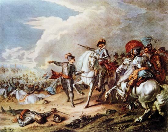
The 17th century was a turbulent time in England. Besides the Civil War (depicted in Figure 1), the period covered by our material saw a number of minor conflicts, such as the Anglo-Spanish Wars and the Thirty Years’ War during the first subperiod and the Anglo-Dutch Wars during the second subperiod. The Civil War between Parliamentarians and Royalists began during Charles I’s reign in 1642. The Parliamentarians executed Charles in 1649, and England was under parliamentary and military rule until 1660. Known as the Interregnum, this period can be broken down into the Commonwealth (1649–1653; the war ended in 1651), the Protectorate (ruled by Oliver Cromwell 1653–1658 and Richard Cromwell 1658–1659) and the second Commonwealth (1659–1660), after which Charles I’s son, Charles II, was restored to the throne.
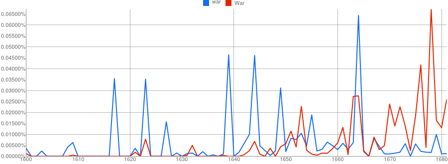
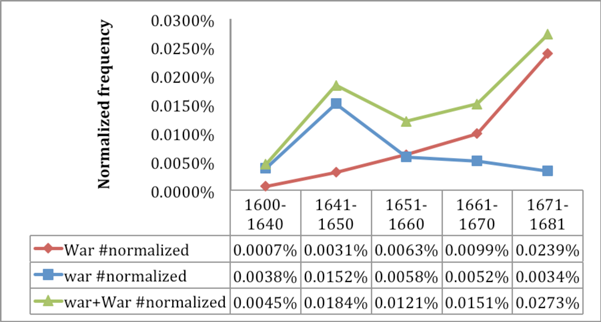
A quick look at the Google Books database, which was also used by Michel et al. (2010), reveals that the use of the word war increases in British English books during the 17th century and that some of the peaks in the frequency coincide with the Civil War (Figure 2). There is a great deal of noise, however, and it is unclear how many of the occurrences actually refer to that particular war.
We also briefly surveyed the underlying data for the Google Books Ngram Viewer and noticed that the corpus is relatively sparsely populated in the 17th century, especially in the period before 1640. For the period 1600–1640, the corpus contains 2.7 million words in 55 books that are spread over only 26 of the 41 years. Thus, for many years there are no samples available, which is not apparent from the Ngram Viewer, where the corresponding years are simply estimated to have a frequency of 0, for any word. The Ngram Viewer provides the possibility to use smoothing, which averages frequencies over several years. However, in the case of sparse data, this smoothing method seems to make things worse rather than better, since sparse regions are then heavily biased towards having lower frequencies.
To increase the reliability, we manually aggregated the data to 5 periods, each of which covers at least 33 books (Figure 3). Notably, in all periods at least half of the books contain the word war. We observe that the frequency of the word war peaks during the Civil War and that the frequency also increases towards the end of the century.
While these results are interesting, they do not tell the whole story. In what follows, we will analyse the entire lexicon of a systematically compiled single-genre corpus, which may yield more reliable results than querying the heterogeneous Google Books with its limited access to data (cf. Davies 2010).
3. Data
Our data set is the normalized-spelling version of the 17th-century part of the Corpus of Early English Correspondence (CEEC; Palander-Collin & Hakala 2011). It consists of 3,055 letters or c. 1.2 million words written in English (as spoken in England) between the years 1600 and 1681. The data set was divided into two c. 40-year periods, 1600–1639 and 1640–1681, motivated by an external event, namely the English Civil War (see Section 2). The first period comprises 1,498 letters or 567,135 words, while the second period consists of 1,557 letters or 656,711 words.
While the corpus is fairly small – the first period is roughly a fifth of the size of the corresponding period in Google Books – it should be large enough for spotting trends, especially when divided in only two subcorpora. The normalized version was used because we wanted to be able to compare word forms rather than spelling variants. The normalization does not extend to morphosyntactic variants; thus, e.g., hath and has have not been collapsed into one form.
The CEEC was compiled in the 1990s by the Sociolinguistics and Language History project team in the Department of English at the University of Helsinki. As the corpus was designed for the purposes of historical sociolinguistics, its sampling unit was the individual letter writer, and an effort was made to create a balanced corpus in terms of gender and social rank, with regional considerations taken into account where possible. Nevertheless, the dominance of men from the upper ranks was unavoidable, as they wrote the most and their letters were considered by posterity important enough to be saved and later published in edited letter collections, on which the corpus is based.
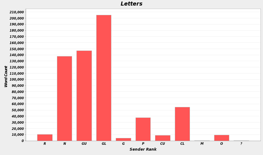
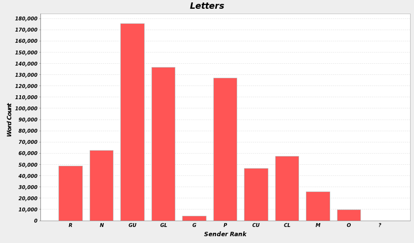
Figures 4 and 5 show the distribution of ranks in the CEEC for our two time periods. The upper ranks are overrepresented, and there is some variation between the periods. While the former period is dominated by letters written by members of the gentry and nobility, the latter period sees a rise in the professional ranks (e.g., lawyers, teachers, medical doctors and army officers), with more material from merchants as well, although the bulk of the writing still comes from the gentry. This needs to be taken into account when interpreting the results.
The standardized-spelling version of the 17th-century part of the CEEC was created in 2011 by members of the CEEC team using the VARD 2 software (Palander-Collin & Hakala 2011; Baron 2011; Baron & Rayson 2009). The normalization was carried out in order to facilitate the use of standard corpus-linguistic tools and methods, such as key word analysis, on the data. In the normalization process, the frequency of word tokens with a variant spelling decreased from 18.2 % to 6.7 %, and that of word types from 56.7 % to 33.8 %. According to Palander-Collin and Hakala (2011), the remaining variation should not have a considerable effect on key word analysis as the token frequency of the variant types is very low.
4. Methods
In Section 5, we study the homogeneity of the corpus over time in quantitative terms, using two statistical methods. In this section, we present technical and practical discussion for both these statistical tests. Sections 4.1 and 4.2 introduce the log-likelihood ratio test and the bootstrap test, and Section 4.3 discusses how to interpret and correct p-values when testing multiple hypotheses at the same time.
4.1 Log-likelihood ratio test
The log-likelihood ratio test (Dunning 1993), sometimes also called the G2 test, is based on the assumption that a text or corpus can be modelled as a sequence of independent Bernoulli trials, i.e., a sequence of random events with binary outcome. This assumes that each word in a corpus is generated independently. In the field of natural language processing, the representation where all words are assumed to be statistically independent is generally known as the bag-of-words model. We will also use this terminology.
The probability distribution for the frequency of an event in a sequence of Bernoulli trials is given by the probability mass function of the binomial distribution. Let K be a random variable representing the frequency of a word in a corpus. If n is the size of the corpus and p the relative frequency of a word, then the probability of observing that word exactly k times in the corpus is given by
\[\text{Pr}(K = k) = {n \choose k} p^k (1-p)^{ n-k}. \qquad \mathbf{(1)} \]
The likelihood function H(p;n,k) is the same as Pr(K = k) in Equation (1); the only difference is that we explicitly mention the parameter p. The log-likelihood ratio test is based on comparing the likelihood ratio λ between two situations, (i) when the two corpora are described using a single parameter p, (ii) when the two corpora are described by two independent parameters p1 and p2 (Dunning 1993):
\[ λ = \frac{\text{max}_pH(p;n_1,k_1)\cdot H(p;n_2,k_2)}{\text{max}_{p_1,\, p_2}H(p_1;n_1,k_1)\cdot H(p_2;n_2,k_2)}. \qquad \mathbf{(2)} \]
The likelihood in situation (ii) is always greater than or equal to the likelihood in situation (i), hence the ratio is always between 0 and 1. Because the test statistic -2 log λ asymptotically follows a χ2 distribution with one degree of freedom, the p-value for the test can be computed by comparing the value of the test statistic to a table of χ2 distributions.
There are other statistical tests based on the bag-of-words model, such as the χ2 test, Fisher’s exact test and the binomial test. For brevity, we do not consider these tests in this paper and we expect these methods to perform very similarly to the log-likelihood ratio test. For further discussion see, e.g., Lijffijt et al. (2011) and Lijffijt et al. (forthcoming).
4.2 Bootstrap test
The bootstrap test (Lijffijt et al. forthcoming) is a non-parametric statistical test based on resampling, which is a statistical method whereby one creates new data sets (in this case corpora) by taking samples (in this case texts) from the original data at random. The idea behind the test is that resampling can be used to estimate the uncertainty in the frequency count of a word q in both corpora, because the resampling introduces small variations to the frequency counts.
The uncertainty of the frequency of a word depends on the dispersion of the word throughout the corpus. If a word is well dispersed, that is, it has approximately equal frequency in all texts, the uncertainty of the estimated frequency is small, but if the word is poorly dispersed, for example, it occurs in only one text, then the uncertainty will be very large.
The p-value has the same meaning as in the log-likelihood ratio test: it is the probability of observing the measured difference in mean frequency under the assumption that the mean frequencies are in fact equal. The difference between the bootstrap test and the bag-of-words tests is that the bootstrap test directly uses the empirical frequency distribution, whereas the bag-of-words tests, such as the log-likelihood ratio test, assume that the frequency distribution is binomial.
The bootstrap test is based on bootstrapping (Efron & Tibshirani 1993), which means that resampling is done with replacement (texts can be included in a ‘random’ corpus multiple times) and the number of samples is equal to the number of samples in the original data. The test operates by producing a series of ‘random’ corpora S1 to SN by repeatedly resampling texts from S, and likewise a series T1 to TN by repeatedly resampling texts from T. For fair comparison, the number of texts in each random corpus is equal to the minimum number of texts in either corpus and the frequency freq(q, Si) is the mean of the normalized frequencies over all texts in the random corpus Si. The p-value is then computed using Equation (3):
\[ p = \frac{1+2\cdot N\cdot\text{min}(p_{one},1-p_{one})}{1+N}, \text{where} \]
\[ p_{one} = \frac{\sum_{i=1}^N H\left(freq(q,T^i)- freq(q,S^i)\right)}{N}, \text{and} \,H(\text{x}) = \left\{ \begin{aligned} 1 \qquad \text{if} \, x \gt 0 \\ 0.5 \qquad \text{if} \, x = 0 \\ 0 \qquad \text{if} \, x \lt 0 \end{aligned} \right.\,. \qquad \mathbf{(3)} \]
The test has one input parameter, N, which is the number of bootstrap samples. A higher N is always better, but one can derive the sufficient N from the required resolution on the p-value. For example, choosing N such that the smallest possible p-value is ten times smaller than the significance threshold α is a safe choice. Since the p-value is an empirical estimate, the smallest p-value that the test can output is 1/(N+1) (Lijffijt et al. forthcoming). Thus, if we use a significance threshold of α = 0.01, then we would like to have 1/(N+1) = 0.01/10 = 0.001, which implies N = 999.
4.3 Interpreting p-values when testing multiple hypotheses
When testing a single hypothesis, the interpretation of a p-value is straightforward: it is the likelihood of observing a measurement, or anything more extreme, under the null hypothesis. Usually, if the p-value for a measurement is sufficiently small, then we reject the null hypothesis. For simplicity, let us choose a significance threshold of α = 0.05. We should be mindful that, when we make a measurement, and the process does follow the null hypothesis, there is (by definition of the p-value) a 5 % probability of observing a p-value of α or less.
Using a significance threshold of 0.05 is fine as long as we test a single hypothesis. Moreover, it is good practice to report the actual p-values rather than just using a threshold, and p-values should not be used as a replacement for studying the underlying data, such as the actual frequencies of occurrence. These and other dangers associated with the use of p-value have been under extensive debate in many social sciences; for an overview see, for example, Krantz (1999). Here we highlight a different problem, that of testing multiple hypotheses.
Under the circumstances described above, there is a 1-α = 0.95 probability of the observation being marked non-significant, assuming that the generative process follows the null hypothesis. Often, it is desirable to maintain this probability, even when testing multiple hypotheses. To illustrate the problem, we give a simple example.
Assume that we are testing 5 hypotheses, instead of one. For each hypothesis the probability that the p-value is lower than or equal to α is α = 0.05 itself. However, the probability that at least one p-value is lower than or equal to α is much higher. We can easily compute the inverse, the probability that all p-values are higher than α: (1-α)^5 = 0.95^5 = 0.774. Thus, the probability that at least one hypothesis is marked as significant is 1 - (1-α)^5 = 1 - 0.774 = 0.226.
This poses a clear danger: if we test enough hypotheses, then we are bound to have many significant findings, even if there is nothing to find. The essential problem here is that the relation between the significance threshold α and the probability of observing p-values that are equal to or lower than α is not that trivial when we are testing multiple hypotheses concurrently.
Statisticians have proposed many methods for correcting p-values so that they are easier to interpret. Two popular metrics used by such correction methods are the Family-Wise Error Rate (FWER) and the False Discovery Rate (FDR). A method that controls the FWER, controls exactly the probability mentioned before, the probability that any p-value is less than or equal to α. A popular and easy method that provides control for the FWER is Bonferroni correction, which is used for example in Oakes and Farrow (2007: 90–91).
However, as noted for example by Oakes and Farrow, Bonferroni correction is a very conservative method and may mark too many interesting results as non-significant. It is often better to provide a control for the FDR, which is the ratio of false positives among all positives. We use here the method introduced in Benjamini and Hochberg (1995), which also introduces the FDR. As shown in this article, the number of falsely accepted hypotheses (type II errors) is often substantially lower compared to methods that control the FWER.
5. A quantitative perspective on stability
We are interested in measuring the stability of the corpus profile over time. An important aspect of the corpus profile is the frequency at which individual words are employed. To study this aspect we conducted a key word analysis between the two periods 1600–1639 and 1640–1681. As discussed in Section 2.2, we expect that there will be some language change, but that the general profile of the corpus remains the same. If this assumption holds, then only a small portion of the words should exhibit a significantly different frequency in the later period, compared to the earlier period. Thus, we can verify this assumption by studying the results of the key word analysis quantitatively.
Our study is inspired by the comparison of several statistical tests in Paquot & Bestgen (2009: 8–17), although the objective in their study is somewhat different. Paquot & Bestgen (2009) compares two corpora (academic texts vs. fiction in the British National Corpus) that are quite dissimilar, such that there would be both spurious and interesting differences, while we hope to find that the two periods are in general fairly comparable. Thus we are interested in similarities as much as differences.
To obtain a thorough view of the differences between the two statistical tests and the possible effects of parameter choices, we computed the number of significant results at different significance thresholds (α = 0.01, α = 0.001, and α = 0.0001) and using various minimum frequency requirements (n ≥ 0, n ≥ 1/100,000, and n ≥ 10/100,000). The results for both tests are given in Tables 1–3. The column marked with ‘Both’ corresponds to the number of words that are significant at the specified level α in both methods. Notice that here we have not yet applied any post-hoc correction for testing multiple hypotheses.
| α |
Log-likelihood ratio |
Bootstrap |
Both |
0.01 |
2,685 (6 %) |
2,365 (5 %) |
2,199 (5 %) |
0.001 |
1,400 (3 %) |
1,209 (3 %) |
1,108 (2 %) |
0.0001 |
937 (2 %) |
759 (2 %) |
722 (2 %) |
Table 1. No minimum frequency (n = 46,440)
| α |
Log-likelihood ratio |
Bootstrap |
Both |
0.01 |
2,365 (37 %) |
2,034 (32 %) |
2,013 (31 %) |
0.001 |
1,400 (22 %) |
1,209 (19 %) |
1,108 (17 %) |
0.0001 |
937 (15 %) |
759 (12 %) |
722 (11 %) |
Table 2. Minimum frequency of 1 per 100,000 words (n = 6,448)
| α |
Log-likelihood ratio |
Bootstrap |
Both |
0.01 |
603 (54 %) |
530 (47 %) |
530 (47 %) |
0.001 |
498 (45 %) |
421 (38 %) |
421 (38 %) |
0.0001 |
432 (39 %) |
354 (32 %) |
354 (32 %) |
Table 3. Minimum frequency of 10 per 100,000 words (n = 1,116)
We observe several trends that are expected: the number of types that have a significantly different frequency in the two periods becomes lower when we choose the significance threshold α more strictly and it also becomes lower if we employ a higher frequency cut-off. Besides, we observe that most of the words that are reported as significant by the bootstrap test are also significant under the log-likelihood ratio test. For example, in Table 3 we observe that all words reported by the bootstrap test are also significant using the log-likelihood ratio test (the numbers for ‘bootstrap’ and ‘both’ are the same).
The question of how much remains the same has several answers. Considering the numbers in Table 1, we could conclude that indeed most types show no variation. However, by comparing Tables 1 and 2, we learn that all types that are significant are also reasonably frequent. Vice versa, it is likely that most types are not significantly different, just because they are very infrequent. It seems that there is little reason to employ a very high frequency cut-off, but a significance threshold of α = 0.01 without post-hoc correction for multiple hypotheses also seems overly optimistic.
Most interesting seem to be the second and third row in Tables 1 (n ≥ 0) and 2 (n ≥ 1 / 100,000), which are the same except that the percentages in Table 2 are higher because of the frequency cut-off. These numbers suggest that there are 759–1,400 types with a significant frequency variation over the two periods, which is 2–3 % of the total types, or 12–22 % of the medium/high-frequency types. The proportion of types that are not significantly different (88 % for the bootstrap test with α = 0.0001) is thus considerably higher than, for example, the numbers reported in Paquot & Bestgen (2009: 11), where they find that only 51.5 % (t-test) or 33.8 % (Wilcoxon rank-sum test) are stable when using the same frequency cut-off as used in Table 2 and a much lower significance threshold (α = 0.000001).
What is also interesting in the results is that the log-likelihood ratio test marks 15–23 % more types as significant compared to the bootstrap test, a difference that is much smaller than in some previous studies (Paquot & Bestgen 2009, Lijffijt et al. forthcoming). Possibly the smaller difference between the two tests is due to the small size of the corpus; e.g., Paquot & Bestgen (2009) is based on two sub-corpora that are almost 25 times the size considered here. If the size matters so much, it remains to be seen whether the perceived comparability is also merely an effect of the small size of the corpus (cf. Hinneburg et al. 2007).
6. Differences between time periods
6.1 Statistical testing in practice
In this section, we study the differences between the two time periods in more detail. All statistical analyses in this section are based on the bootstrap test, since that has been shown to be the most appropriate statistical test for the type of comparison exercised here (Lijffijt et al. forthcoming). In order to use the statistical test, we still have to select a significance threshold and optionally choose to use minimum frequency cut-off.
We have chosen to set the significance threshold to α = 0.05 and use the Benjamini-Hochberg procedure to correct for the large amount of tested hypotheses. The Benjamini-Hochberg procedure outputs a corrected threshold, such that the original α gives the ratio of false positives over all results that are significant (see Section 4.3 for more details). The corrected significance threshold is α = 0.0016, which is slightly higher than the lowest threshold studied in Section 5. In comparison to some earlier studies, this threshold is relatively high, for example, Paquot & Bestgen (2009: 11) use α = 0.000001 and Oakes & Farrow (2007: 91) use α = 0.000000001961. Although the threshold is relatively high, it still guarantees that with high probability (1 - α = 0.95) the significant results are true positives.
A practical problem that is often encountered when comparing corpora is that the number of types that are significantly different can be very large, prohibiting a comprehensive interpretation of the results. In Section 5, we found that the statistical tests inherently have a minimum frequency threshold, and from a statistical perspective, there is no need to impose any minimum frequency constraints. We found that there are 1,292 words whose frequency is significantly different between the two time periods, which is already quite a challenge to interpret. Based on a first look at the data, we pursued two lines of exploration of the significant differences: in Section 6.2 we study language change among frequent words, that is words with a frequency of at least 100 per 100,000, and in Section 6.3, we study words that are related to the Civil War, without imposing any frequency constraints.
6.2 The Civil War effect and linguistic change in progress
We followed earlier studies in limiting the number of items to be analysed and first zoomed in on the most frequent items with significantly different distributions in the two data sets according to both tests. More specifically, the significant items had to have a normalized frequency of at least 100 per 100,000 words in both subcorpora; there were 51 of these (a list of them is available for download as a comma-separated file below). Rather than arguing for large-scale cultural processes of stylistic change such as colloquialization, we traced more local causes behind the variation between the two 40-year periods. More data were needed to observe potential reflections of current affairs or cultural shifts in the subcorpora (see 6.3).
(Download the complete analysis file – comma-separated values, .CSV file).
Certain differences between the two lists reflect ongoing processes of language change. One of them is the degree adverb very, which stands out in the second period. Earlier studies using the Helsinki Corpus show that very is gaining momentum in the 17th century in the intensifier function (Nevalainen 1997: 174). It can be found in most letters of the period, as in example (1), written by Frances Hatton to her husband. (All examples are cited from the modern spelling version of the CEEC, which normalizes all spelling variants whose minimum frequency is 40 or above.)
| (1) |
My dear Lord, I should be very glad you would bring some chocolate along with you. I hope I shall receive a good account of all your business, for I long to know. My daughter Nany is very well, and was yesterday at my Lord Brudnal’s. I believe I shall like your cook very well. |
|
(Frances Hatton, 1677; HATTON I, 148) |
Other clear indicators of change in progress are hath and doth, both overrepresented in the first period, as opposed to has, which is overrepresented in the second period. What can be detected here is the spread of the 3rd-person present-tense suffix -s to these high-frequency verbs (Nevalainen & Raumolin-Brunberg 2003: 67–68). The older forms prevail in the first decades of the 17th century but lose out to the incoming ones in the second half. As changes take time, the older forms are still found in the second period as well. In (2), Isaac Basire Junior is writing to his father in 1666 and uses has, whereas his mother Frances Basire writing to her husband ten years earlier used hath (3).
| (2) |
Mr. Rushworth has been very busy, and not to be met with. To-morrow morning we are to meet at his house in Danby Lane, in the Strand. |
|
(Isaac Basire Jr, 1666; BASIRE, 249) |
| (3) |
My earnest desire is that I may have one of our with my friend Busby, which I could not have all this tim for want of a carten a lowans from you, being all most 4 years and receiving but 22 pounds from you, it hath gone very hard with me ... |
|
(Frances Basire, 1655; BASIRE, 138) |
Other shifts in verbal usage in the 17th century include the generalization of the auxiliary do in negative contexts (Nurmi 1999), and the spread of can/could at the expense of may/might (e.g., Kytö 1991). Similarly, are is established as the regular indicative plural of the verb be throughout the country as the southern be plural is being phased out (Nevalainen 2000).
While these changes are supported by earlier research and so offer plausible explanations for over- or underrepresentation of their respective indicators in the data, other cases are less clear-cut in that they index polyfunctional word forms. They may nevertheless be to some extent indicative of changes in progress. These include the overrepresentation of which in the first period and of who in the second. The wh-relative pronoun system was undergoing change as the subject form who was gaining ground with human antecedents at the expense of which (Nevalainen 2012). The examples in (4) and (5) come from the letters of two upper-ranking women writing to their family in the early and mid-17th century, respectively.
| (4) |
I can do no less then with all dilligenc and expedition seek to obtain the effeckt of that: which both your self and all others. which hath heard of this matter. doth Judge to be both reasonable and consionable:/ |
|
(Katherine Paston, 1618; KPASTON, 44) |
| (5) |
The banes between my Lord of Chesterfeild and his mistress was forbidden in the church after they were twice asked by a Lady who pretends he is engaged to her: what will be the issue of it I do not yet know. |
|
(Anne Conway, 1657; CONWAY, 141) |
Interesting though it is, one would not want to draw any far-reaching conclusions on the overrepresentation of the pronoun she in the second period. The 3rd-person neuter pronoun it is similarly more prominent in the second subcorpus, and so are the 3rd-person plural forms they, them and their. No diachronic change is reported for these pronouns in the literature and one would not want to make much of this variation between the subcorpora without breaking the data into sociolinguistically more meaningful subsets (see further Säily, Nevalainen & Siirtola 2011).
6.3 The Civil War effect in vocabulary
Apart from the topics treated by the individual letter-writers in their correspondence, which fall outside the scope of this study, various broader issues in 17th-century England could be reflected in the data, including major historical events such as the English Civil War. We decided to focus on war-related vocabulary.
We manually went through the entire list of words that were significantly overused in either period according to both methods, and checked promising items against the Society > Armed Hostility section of the Historical Thesaurus of the Oxford English Dictionary (HT). Outside the HT, some proper nouns and the word restoration were also included. This resulted in a list of 70 possibly war-related words, which is available for download as a comma-separated file below.
We then studied the actual instances in context and determined that 35 of these words had something to do with war in at least some of the cases. Out of these words, 34 were overused during the latter period (which is when the Civil War occurred) and only one, mariners, in the former period. Furthermore, only a couple of the instances of mariners were actually war-related, so the overuse was probably not due to war. The clearest examples of war-related overuse in the latter period were the words armies, colonel, militia, officers, ordnance, regiment, restoration and war.
(Download the complete analysis file – comma-separated values, .CSV file.)
A further examination of the 34 words overused in the latter period confirmed that at least some of the instances of each word were related to the Civil War or its aftermath. Others, however, dated from the Restoration onwards, so it might have been useful to split the period in half to determine how much of the overuse could be explained by the Civil War and how much by later wars. In any case, a great deal of the overuse could be linked to a few specific persons, such as Colonel John Jones (6), parliamentarian army officer and regicide, who was nominated Commander-in-Chief in Ireland in 1659 (Roberts 2004).
| (6) |
As touching the l’re sent to Scotland it was mine only, as a Servant to the Army, drawn by the direction of the Officers present, and signed by them with my self, and I cannot find that any thing in it disrespects the Parliamt, or public safety which is above Parliamts, that our Armies should engage against one another in blood.
(John Jones, 1659; JONES, 282) |
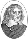
Figure 7. Portrait of John Jones. From Plant (2005).
|
Another frequent war correspondent was Nehemiah Wharton (7), a parliamentarian officer in the Earl of Essex’s army, who wrote to his previous employer, George Willingham, a merchant in London.
| (7) |
It is very poor, for many of our soldiers can get neither beds, bread, nor water, which makes them grow very strong, for backbiters have been seen to march upon some of them six on breast and eight deep at their open order, and I fear I shall be in the same condition e’er long, for we can get no carriage for officers, so that my trunk is more slighted than any other, which is occasioned, as I conceive, partly by the false informations of Lieut.-Col. Briddeman and our late Sergeant Major General Ballard, profane wretches; but chiefly for want of our Colonel, who should be one of the Council of War, at which Council we have none to plead for us or remove false aspersions cast upon us, in so much that I have heard some of our captains repent their coming forth, and all for want of a Colonel. |
|
(Nehemiah Wharton, 1642; WHARTON, 18) |
Women, too, wrote about the war, as in example (8), an excerpt from a letter by a gentlewoman, Dorothy Osborne, to her future husband, William Temple; she had lost two brothers in the war (Parker 2004).
| (8) |
if I am not mistaken that Monk has a brother lives in Cornwell, an honest Gentleman I have heard, and one that was a great acquaintance of a Brother of mine who was killed there during the War, and so much his friend that upon his death he put himself and his Family into mourning for him, which is not usual I think where there is no relation of kindred.
(Dorothy Osborne, 1653; OSBORNE, 81) |
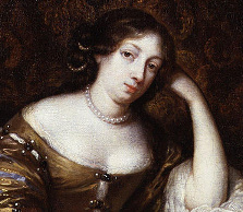
Figure 8. Dorothy, Lady Temple (detail), by Gaspar Netscher, 1671. From Wikimedia Commons. |
7. Discussion
Comparing our findings with previous studies is hampered by the scarcity of past work on diachronic corpora. One of the few diachronic studies of vocabulary stability and change is Baker (2011), but for various reasons it is not directly comparable with ours. Baker analysed the 75-year period covered by the British branch of the Brown family of corpora and included words whose absolute frequency was more than 1,000 instances in the four corpora added together. Altogether 380 words met this criterion, covering 62 % of the total vocabulary in the four corpora.
Baker’s analysis of the stability and change of words was based on their coefficient of variance (CV), which is derived from their standard deviation (SD) scores. As one might expect, the stable ‘lockwords’ which do not exhibit change include a large number of function words, including are, can/could, do; have, had; what and who (all more frequent than expected in the second period in the CEEC data), whereas decrease is detected in may, must, shall, should; which, whose, and the intensifier very. These recessive items could be linked with ongoing change in the language.
Baker’s results are interesting but, because of methodological choices, difficult to compare not only with our study but with previous research more generally. Setting cut-off points and frequency limits to the items discussed is a practical necessity in word-frequency studies but makes cross-study comparisons less straightforward. This problem can be to some extent circumvented by appending the word-frequency data analysed to the publication, as we have done here.
Oakes and Farrow (2007) raise another issue that complicates word-frequency comparisons across corpora for the purpose of comparing cultural differences. Although some are structurally comparable, the available databases have not been compiled with comparative vocabulary studies in mind, and are therefore less than ideally suited for that purpose. Hence the findings based on them should not be overgeneralized.
Our method of classifying vocabulary as war-related differs from Leech and Fallon’s (1992) approach in that we checked our intuitions against the HT. This provides greater objectivity but limits the kinds of words that were included; for instance, there were some emotion words which could have been war-related but which were not taken into consideration because they were not found under the Society > Armed Hostility section of the HT.
In Section 2.2 above, we tentatively explored the Civil War effect using the Google Books Ngram Viewer. Even though the data were noisy, they seemed to indicate an effect similar to our CEEC data. We conclude that this online tool can be a useful heuristic in studies of this kind, but that the results should be checked against more reliable data using significance testing. One way to improve the reliability of the Google Books data is to analyse the actual n-gram frequencies aggregated over longer time periods. In our case they show that the first 40-year period is quite poorly represented in the Google Books database. The second period is more comprehensive, and does confirm the overall increase in the use of war shown in Figure 2.
A serious obstacle to comparing word-frequency studies is the wide range of variation in the statistical measures used in testing the significance of results obtained across corpora. Our point of departure for this study was the fact that the application of chi-square and log-likelihood ratio tests, widely used in past research, can be challenged on the grounds that they are based on the assumption that words are distributed randomly in texts (Kilgarriff 2005). To show that significance tests based on different assumptions also yield different results, we compared the log-likelihood ratio test with the bootstrap method. The log-likelihood ratio test is expected to produce many more significant differences than the bootstrap method, and that also proved to be the case with our single-genre data, although to a lesser extent than in larger corpora.
Similarly, Lijffijt et al. (forthcoming) found clear differences between several methods of significance testing when they were applied to male and female writing in the prose fiction subcorpus of the British National Corpus. In the present study, our hypotheses were more exploratory and our data less abundant; furthermore, as noted by Oakes & Farrow (2007: 85), variation in the content of texts can obscure cultural key words. These are common problems especially when corpora that are strictly stratified across a range of topics and genres are used for detecting cultural key words. Nevertheless, we believe that the standardization of methods is an aim worth striving for: as the bootstrap test has been reliably proved better than a number of other tests by Lijffijt et al. (forthcoming) with a large corpus (the BNC), it should also be used with smaller corpora, even though the results might be less striking.
An issue to consider with the bootstrap test concerns the unit of sampling: what constitutes an independent text? In this study we have used individual letters as texts, but a case could be made for sampling all letters written by a person during a certain time period (see Evans 2012, Malmgren et al. 2009, Nevalainen & Raumolin-Brunberg 2003), or even all letters written by two correspondents to each other in a given time period (Fitzmaurice 2002).
If a phenomenon is robust enough, however, it is likely to show up regardless of how the sampling unit is defined; when the samples are more dependent on each other, there will simply be more noise in the results. In any case, text-level independence is always a more reasonable assumption than the word-level independence assumed by the bag-of-words tests, which means that the bootstrap test will yield fewer misleading results for the scholar to wade through than, say, the log-likelihood ratio test.
Although the bootstrap test is already available for statistical and computing software such as R and Matlab (Lijffijt 2012), we hope it will also be integrated into software packages intended specifically for corpus linguists, making the method accessible to everyone in the field.
8. Conclusion
We set out to explore the question of diachronic stability within a historical single-genre corpus of personal correspondence. We found that the two subperiods of the CEEC that we examined were reasonably similar to each other with regard to their lexis, more so than bag-of-words methods of significance testing would lead us to assume. In addition to the method, the degree of similarity observed depends on several factors, including the size of the corpus as well as the type of post-hoc correction, frequency cut-off and significance threshold used.
We also discovered that the differences between the time periods are not arbitrary. Rather, our method makes it possible to find both linguistic changes in progress (Section 6.2) and changes in cultural vocabulary that are explainable in terms of the historical events and cultural phenomena of the period (Section 6.3). In our test case, the English Civil War, some of the changes in cultural vocabulary could also be due to the composition of the corpus: although both periods were dominated by the gentry, in the period 1640–1681 there is an increase in letters written by professional people, mostly military personnel. Then again, this reflects what was happening at the time, as many men were recruited into the opposing armies and these events affected the population at large.
Acknowledgements
This work was supported in part by the Academy of Finland grant 129282 to the DAMMOC project, the Finnish Doctoral Programme in Computational Sciences (FICS) and by Langnet, the Finnish Graduate School in Language Studies, as well as by the Academy of Finland’s Academy professorship scheme. The authors would like to thank the participants at the Helsinki Corpus Festival and the DAMMOC team for useful comments and discussions, and an anonymous reviewer for helpful feedback. The first two authors contributed equally to this work.
Sources and software
Baron, Alistair. 2011. VARD 2. http://www.comp.lancs.ac.uk/~barona/vard2/
Davies, Mark. 2010. “The Corpus of Historical American English, Google Books, and our new Google Books interface”. http://corpus.byu.edu/coha/compare-googleBooks.asp
English Civil War, in Wikipedia, the Free Encyclopedia, http://en.wikipedia.org/wiki/English_Civil_War
HT = Historical Thesaurus of the Oxford English Dictionary. 2009. Edited by Christian Kay, Jane Roberts, Michael Samuels & Irené Wotherspoon. OED Online. http://www.oed.com/thesaurus
Lijffijt, Jefrey. 2012. Bootstrap test for R and Matlab. http://users.ics.aalto.fi/lijffijt/bootstraptest/
Palander-Collin, Minna & Mikko Hakala. 2011. “Standardized versions of the Corpora of Early English Correspondence”. http://www.helsinki.fi/varieng/CoRD/corpora/CEEC/standardized.html
Plant, David. 2005. “Biography of John Jones”. British Civil Wars and Commonwealth website. http://www.british-civil-wars.co.uk/biog/john-jones.htm
Scott, Mike. 2012. WordSmith Tools. http://www.lexically.net/wordsmith/
References
Baker, Paul. 2011. “Times may change, but we will always have money: Diachronic variation in Recent British English”. Journal of English Linguistics 39(1): 65–88. doi:10.1177/0075424210368368
Baron, Alistair & Paul Rayson. 2009. “Automatic standardisation of texts containing spelling variation: How much training data do you need?” Proceedings of the Corpus Linguistics Conference: CL2009, University of Liverpool, UK, 20–23 July 2009, ed. by Michaela Mahlberg, Victorina González-Díaz & Catherine Smith. http://ucrel.lancs.ac.uk/publications/cl2009/ (article #314)
Benjamini, Yoav & Yosef Hochberg. 1995. “Controlling the false discovery rate: A practical and powerful approach to multiple testing”. Journal of the Royal Statistical Society: Series B (Methodological) 57(1): 289–300. http://www.jstor.org/stable/2346101
Biber, Douglas & Edward Finegan. 1997. “Diachronic relations among speech-based and written registers in English”. To Explain the Present: Studies in the Changing English Language in Honour of Matti Rissanen,ed. by Terttu Nevalainen & Leena Kahlas-Tarkka, 253–275. Helsinki: Société Néophilologique.
CEEC = Corpus of Early English Correspondence. 1998. Compiled by Terttu Nevalainen, Helena Raumolin-Brunberg, Jukka Keränen, Minna Nevala, Arja Nurmi & Minna Palander-Collin at the Department of English, University of Helsinki. http://www.helsinki.fi/varieng/CoRD/corpora/CEEC/
Church, Kenneth W. & William A. Gale. 1995. “Poisson mixtures”. Natural Language Engineering 1(2): 163–190. doi:10.1017/S1351324900000139
Dunning, Ted. 1993. “Accurate methods for the statistics of surprise and coincidence”. Computational Linguistics 19(1): 61–74. http://aclweb.org/anthology-new/J/J93/
Efron, Bradley & Robert J. Tibshirani. 1993. An Introduction to the Bootstrap. New York: Chapman & Hall.
Evans, Melanie. 2012. “A sociolinguistics of early modern spelling? An account of Queen Elizabeth I’s correspondence”. This volume. http://www.helsinki.fi/varieng/journal/volumes/10/evans
Evert, Stefan. 2006. “How random is a corpus? The library metaphor”. Zeitschrift für Anglistik und Amerikanistik 54(2): 177–190. http://www.zaa.uni-tuebingen.de/?attachment_id=825
Fitzmaurice, Susan M. 2002. The Familiar Letter in Early Modern English: A Pragmatic Approach. Amsterdam & Philadelphia: John Benjamins.
HC = The Helsinki Corpus of English Texts. 1991. Compiled by Matti Rissanen (Project leader), Merja Kytö (Project secretary); Leena Kahlas-Tarkka, Matti Kilpiö (Old English); Saara Nevanlinna, Irma Taavitsainen (Middle English); Terttu Nevalainen, Helena Raumolin-Brunberg (Early Modern English). Department of English, University of Helsinki. http://www.helsinki.fi/varieng/CoRD/corpora/HelsinkiCorpus/
Hinneburg, Alexander, Heikki Mannila, Samuli Kaislaniemi, Terttu Nevalainen & Helena Raumolin-Brunberg. 2007. “How to handle small samples: Bootstrap and Bayesian methods in the analysis of linguistic change”. Literary and Linguistic Computing 22(2): 137–150. doi:10.1093/llc/fqm006
Hofland, Knut & Stig Johansson. 1982. Word Frequencies in British and American English. Bergen: Norwegian Computing Centre for the Humanities/London: Longman.
Hundt, Marianne & Christian Mair. 1999. “‘Agile’ and ‘uptight’ genres: The corpus-based approach to language change in progress”. International Journal of Corpus Linguistics 4(2): 221–242. doi:10.1075/ijcl.4.2.02hun
Katz, Slava M. 1996. “Distribution of content words and phrases in text and natural language modelling”. Natural Language Engineering 2(1): 15–59. doi:10.1017/S1351324996001246
Kilgarriff, Adam. 1996. “Which words are particularly characteristic of a text? A survey of statistical approaches”. Proceedings of the AISB Workshop on Language Engineering for Document Analysis and Recognition, 33–40. Sussex University. http://www.kilgarriff.co.uk/Publications/1996-K-AISB.pdf
Kilgarriff, Adam. 2001. “Comparing corpora”. International Journal of Corpus Linguistics 6(1): 97–133. doi:10.1075/ijcl.6.1.05kil
Kilgarriff, Adam. 2005. “Language is never, ever, ever, random”. Corpus Linguistics and Linguistic Theory 1(2): 263–276. doi:10.1515/cllt.2005.1.2.263
Krantz, David H. 1999. “The null hypothesis testing controversy in psychology”. Journal of the American Statistical Association 94: 1372–1381.
Kytö, Merja. 1991. Variation and Diachrony, with Early American English in Focus: Studies on can/may and shall/will (Bamberger Beiträge zur Englischen Sprachwissenschaft). Frankfurt am Main: Peter Lang.
Leech, Geoffrey & Roger Fallon. 1992. “Computer corpora – What do they tell us about culture?” ICAME Journal 16: 29–50. http://icame.uib.no/journal.html
Lijffijt, Jefrey, Panagiotis Papapetrou, Kai Puolamäki & Heikki Mannila. 2011. “Analyzing word frequencies in large text corpora using inter-arrival times and bootstrapping”. Proceedings of ECML-PKDD 2011 – Part II, ed. by Dimitrios Gunopulos, Thomas Hofmann, Donato Malerba & Michalis Vazirgiannis, 341–357. Berlin: Springer-Verlag. doi:10.1007/978-3-642-23783-6_22
Lijffijt, Jefrey, Terttu Nevalainen, Tanja Säily, Panagiotis Papapetrou, Kai Puolamäki & Heikki Mannila. Forthcoming. “Significance testing of word frequencies in corpora”.
Malmgren, R. Dean, Daniel B. Stouffer, Andriana S.L.O. Campanharo & Luís A. Nunes Amaral. 2009. “On universality in human correspondence activity”. Science 325(5948): 1696–1700. doi:10.1126/science.1174562
Michel, Jean-Baptiste, Yuan Kui Shen, Aviva Presser Aiden, Adrian Veres, Matthew K. Gray, The Google Books Team, Joseph P. Pickett, Dale Hoiberg, Dan Clancy, Peter Norvig, Jon Orwant, Steven Pinker, Martin A. Nowak & Erez Lieberman Aiden. 2010. “Quantitative analysis of culture using millions of digitized books”. Science 331(6014): 176–182. doi:10.1126/science.1199644
Nevalainen, Terttu. 1997. “The processes of adverb derivation in Late Middle and Early Modern English”. Grammaticalization at Work: Studies of Long-term Developments in English (Topics in English Linguistics 24), ed. by Matti Rissanen, Merja Kytö & Kirsi Heikkonen, 145–190. Berlin & New York: Mouton de Gruyter. doi:10.1515/9783110810745.145
Nevalainen, Terttu. 2000. “Processes of supralocalisation and the rise of Standard English in the Early Modern period”. Generative Theory and Corpus Studies: A Dialogue from 10 ICEHL (Topics in English Linguistics 31), ed. by Ricardo Bermúdez-Otero, David Denison, Richard M. Hogg & C.B. McCully, 329–371. Berlin & New York: Mouton de Gruyter. doi:10.1515/9783110814699.329
Nevalainen, Terttu. 2008. “Variation in written English: Grammar change or a shift in style?” Socially-Conditioned Language Change: Diachronic and Synchronic Insights, ed. by Susan Kermas & Maurizio Gotti, 31–51. Lecce: Edizioni del Grifo.
Nevalainen, Terttu. 2012. “Reconstructing syntactic continuity and change in Early Modern English regional dialects: The case of who”. Analysing Older English, ed. by David Denison, Ricardo Bermúdez-Otero, Christopher McCully & Emma Moore, with the assistance of Ayumi Miura, 159–184. Cambridge: Cambridge University Press. doi:10.1017/CBO9781139022170.015
Nevalainen, Terttu & Helena Raumolin-Brunberg. 2003. Historical Sociolinguistics: Language Change in Tudor and Stuart England (Longman Linguistics Library). London: Pearson Education.
Nurmi, Arja. 1999. A Social History of Periphrastic do (Mémoires de la Société Néophilologique de Helsinki 56). Helsinki: Société Néophilologique.
Oakes, Michael P. & Malcolm Farrow. 2007. “Use of the chi-squared test to examine vocabulary differences in English-language corpora representing seven different countries”. Literary and Linguistic Computing 22(1): 85–100. doi:10.1093/llc/fql044
Paquot, Magali & Yves Bestgen. 2009. “Distinctive words in academic writing: A comparison of three statistical tests for keyword extraction”. Corpora: Pragmatics and Discourse, ed. by Andreas H. Jucker, Daniel Schreier & Marianne Hundt, 247–269. Amsterdam & New York: Rodopi. http://www.ingentaconnect.com/content/rodopi/lang/2009/00000068/00000001/art00013
Parker, Kenneth. 2004. “Osborne, Dorothy [married name Dorothy Temple, Lady Temple] (1627–1695)”. Oxford Dictionary of National Biography, online edition, ed. by Lawrence Goldman. Oxford: Oxford University Press. doi:10.1093/ref:odnb/27109
Raumolin-Brunberg, Helena. 1998. “Social factors and pronominal change in the seventeenth century: The Civil-War effect?” Advances in English Historical Linguistics (1996) (Trends in Linguistics: Studies and Monographs 112), ed. by Jacek Fisiak & Marcin Krygier, 361–388. Berlin: Mouton de Gruyter. doi:10.1515/9783110804072.361
Rayson, Paul. 2008. “From key words to key semantic domains”. International Journal of Corpus Linguistics 13(4): 519–549. doi:10.1075/ijcl.13.4.06ray
Rayson, Paul, Damon Berridge & Brian Francis. 2004. “Extending the Cochran rule for the comparison of word frequencies between corpora”. Le poids des mots: Proceedings of the 7th International Conference on the Statistical Analysis of Textual Data (JADT 2004), ed. by Gérald Purnelle, Cédrick Fairon & Anne Dister, 926–936. Louvain-la-Neuve: Presses universitaires de Louvain. http://lexicometrica.univ-paris3.fr/jadt/jadt2004/pdf/JADT_090.pdf
Rayson, Paul, Geoffrey Leech & Mary Hodges. 1997. “Social differentiation in the use of English vocabulary: Some analyses of the conversational component of the British National Corpus”. International Journal of Corpus Linguistics 2(1): 133–152. doi:10.1075/ijcl.2.1.07ray
Roberts, Stephen K. 2004. “Jones, John (c.1597–1660)”. Oxford Dictionary of National Biography, online edition, ed. by Lawrence Goldman. Oxford: Oxford University Press. doi:10.1093/ref:odnb/15026
Säily, Tanja, Terttu Nevalainen & Harri Siirtola. 2011. “Variation in noun and pronoun frequencies in a sociohistorical corpus of English”. Literary and Linguistic Computing 26(2): 167–188. doi:10.1093/llc/fqr004
Smitterberg, Erik. 2008. “The progressive and phrasal verbs: Evidence of colloquialization in nineteenth-century English?” The Dynamics of Linguistic Variation: Corpus Evidence on English Past and Present, ed. by Terttu Nevalainen, Irma Taavitsainen, Päivi Pahta & Minna Korhonen, 269–289. Amsterdam & Philadelphia: John Benjamins.
|
|

