Studies in Variation, Contacts and Change in English
Studies in Variation, Contacts and Change in English
Joseph Flanagan
University of Helsinki
This paper presents various strategies designed to make analyses involving big, medium, or small data reproducible and show how they can be implemented in RStudio, an IDE (integrated development environment) for the statistical programming language R. While these tools and practices have become increasingly common in certain fields and disciplines, they are not yet widely known – let alone practiced – within the humanities. I will conclude the paper with some thoughts about the obstacles preventing the strategies I outline from becoming standard practice within the humanities and will offer some suggestions for how we might overcome those obstacles.
In a blog post entitled, “Adventures in Correcting the (Semi-)Scientific Record” (Carey 2014b), Ray Carey, then a post-graduate at the University of Helsinki, wrote about his experiences in trying to correct an “obvious error” in Hilary Nesi’s Laughter in University Lectures (2012). While the documentation for the British Academic Spoken English corpus (BASE), one of the corpora used in the article, reports a word count of just over 1.6 million words, Nesi reports that the four genres that make up the corpus total 2,646,920 words in all (2012: 3, 83). Noting that such a large difference would affect the normalized frequency of laughter reported in the paper and thus its findings concerning the relative lack of laughter in the BASE lecture subcorpus compared with the Michigan Corpus of Academic Spoken English (MICASE), Carey wrote to Nesi asking about the discrepancy. He received no reply. Carey then downloaded the XML version of the corpus and tried to reproduce Nesi’s figures using various methods, including counting XML tags as words, but was unable to do so (Carey 2013). Carey then published a reader response (2014a) to Nesi’s article, once again noting the discrepancy, providing his own normalized frequency for laughter in the BASE corpus, and showing that the difference in frequency of laughter in BASE and MICASE lectures largely disappears with the corrected word count. [1] Nesi’s response (2014) thanks Carey for correcting the calculations but provides no additional information about how the mistaken word count occurred in the first place. To this day, it remains unclear how the error occurred (and the figures in Nesi’s article remain uncorrected).
I cite this anecdote not to cast aspersions on Nesi or her work. Indeed, the response of any researcher to Nesi’s predicament should not be self-satisfied smugness but a sense of “there but for the grace of God go I”. It is depressingly easy for a mistake to creep into an analysis and go unnoticed. Many researchers would find it difficult – if not impossible – to reproduce the graphs, tables, and/or statistical results of a study years after the research was completed. Indeed, I invite you to randomly select one of your publications from a few years ago. Would you be able to reproduce your results today? If so, how long would it take and how difficult would it be? If not, would you still believe in the validity of your results? Would you expect readers to do so?
An earlier version of this paper was read at a conference entitled “From data to evidence”. I want to use the exchange between Nesi and Carey to point out that what we typically describe as “evidence” is often merely a claim made by a particular researcher. This tendency to mischaracterize claims as evidence is related to what Ted Pedersen refers to as “the paradox of faith-based empiricism” (2008). “Results must be supported experimentally with great precision and detail and are judged according to harsh empirical standards”, he writes, “but we as readers and reviewers are asked to accept that these results are accurate and reproducible on faith” (Pedersen 2008: 469–470). This acceptance of the accuracy and reliability of cited evidence in the form of tables, figures, and statistics has become almost routine for both readers (who perhaps can be forgiven for believing that the peer review process makes the reported findings reliable) and peer reviewers and editors (whose faith in the accuracy of the reported evidence is less understandable). Again, I invite you to think about an article whose results you cited as evidence in favour of your position. Have you checked the validity of the results by reproducing them yourself? Could you even do so? If not, on what basis do you think those results count as “evidence” for your own position?
If we want to consider the results published in papers as “evidence”, then, a minimal criterion should be that those results are reproducible. By reproducible, I mean that an interested person would be able to easily and exactly reproduce every statistic, table, and figure found in the paper working from the rawest form of the data. [2] Admittedly, we are still far from the stage where it is possible to easily reproduce most kinds of linguistic research: manual annotations of the data and manual corrections of automated annotation are still needed for many – if not most – of the kind of analyses linguists perform, and it is debatable whether manual annotations can ever achieve full reproducibility. Still, the fact that full reproducibility is not possible does not mean that we should abandon ourselves to faith-based empiricism: there is a whole spectrum of possibilities between the extremes of full reproducibility and no reproducibility.
This paper and accompanying videos are intended to introduce some strategies, tools, and workflows that, if widely available, would make it easy for others to accomplish a limited form of reproducibility: the ability to reproduce the statistics, tables, and figures that appear in a published paper once the necessary manual annotations and corrections of the data have taken place. [3] In order to avoid simplifying the issue by working with toy data, I will show how to reproduce part of Wolk et al. (2013), a study of the genitive and dative alternation in the ARCHER corpus (Biber et al. 1994). My aim here is not to check their work, and I have accordingly not indicated any issues arising from my efforts to reproduce it. Indeed, Wolk et al. (2013) should be commended for providing both the data and the code that made my efforts to reproduce their work possible in the first place. [4] Instead, I want to use my experience attempting to reproduce their work to formulate six general principles for creating reproducible research and to demonstrate how those principles can be put into action using RStudio, a free and open-source integrated development environment (IDE) for the statistical programming language R. While these tools are thus very much R centered, the underlying strategies and concerns have wider application.
My paper also practices what it preaches. This paper can be reproduced in its entirety from the repository on Bitbucket, along with additional figures and statistical models from Wolk et al. (2013).
A short outline of these strategies is listed below:
There are generally a large number of steps that lead from the raw data to a final result that appears in the form of a statistic, table, or figure. At the very least, the data needs to be transformed into a format that can be read by whatever software or programming environment performs the analysis. The data often need to be cleaned of errors, missing values must be dealt with, new variables need to be created, observations may be excluded from analysis, and countless other tasks performed. I will call the full sequence of steps – whether automated or performed manually – a data analysis pipeline. Within this pipeline, the results of some of these steps are visible, while others are merely intermediary, serving as the transitory input for a more visible step in the pipeline. For instance, we may wish to stem a word and include only frequent stems in a regression model, coding those that are less than four as OTHER. In this instance, the result of the stemming of frequent words is visible, whereas the stemming of infrequent words is not: since infrequent words are coded as OTHER, we know that the frequency is less than four but not the precise form of the stem.
Reproducing a final result thus means that it is possible for someone to reproduce each step of the data analysis pipeline, moving from the raw data, through the intermediate data, to the final results. In order reproduce each of these steps, it is thus essential that the raw data be preserved in its original form, since overwriting the original data set means that at least one of the steps in the data analysis pipeline has been erased. It is also crucial that the full sequence of steps in the data analysis pipeline are recorded and not only those that are visible. It is here that a programming environment like R or Python is vastly superior to Graphical User Interface (GUI) software packages where users click through drop-down menus. For instance, here is how we can create a new variable containing the stem of lexical words that have a frequency greater than 4:
# Create a stemmed theme head variable, with stems less than 4 coded as OTHER
datives2 <- datives %>% # Create new dataset here so we don't overwrite existing one
mutate(prunedThemeHead = tolower(themeHead),
prunedThemeHead = wordStem(prunedThemeHead)) %>%
group_by(prunedThemeHead) %>%
mutate(frequency = n()) %>%
ungroup() %>%
mutate(prunedThemeHead = replace(prunedThemeHead, frequency < 4, "OTHER"))
and this produces the following (for the first ten values):
## # A tibble: 3,093 × 3
## themeHead frequency prunedThemeHead
## <chr> <int> <chr>
## 1 me 15 me
## 2 rent 3 OTHER
## 3 eye 3 OTHER
## 4 Sum 12 sum
## 5 us 10 u
## 6 petrol 1 OTHER
## 7 much 11 much
## 8 compliment 13 compliment
## 9 job 3 OTHER
## 10 tribute 7 tribut
## # ... with 3,083 more rows
While it is technically possible to make analyses in GUI programs reproducible by manually noting all the operations that were performed, it is all-too-easy for the documentation to become out-of-sync with how the final result was actually produced. And once the documentation becomes out-of-sync, the only way the final result can be reproduced is by repeating the whole data analysis pipeline from scratch, a labor-intensive and tedious process that few would be bothered to undertake. [5] By instead specifying the data analysis pipeline in the form of code that can directly executed, we can ensure that documentation matches the data analysis pipeline that generated the final results. Indeed, reproducing that pipeline is as simple as running the code, since the pipeline is the code. [6]
Once we realize that our code is the medium of our documentation, it becomes important to write code in such a way that others can make sense of it. Comments that explain what a code block does or clarify ambiguous lines help others (as well as your future self) understand the code. Since it can become easy for comments or documentation to the code to become out-of-sync with the code itself (e.g., you make improvements to the code and forget to update the accompanying documentation), code should ideally be self-documenting. Use the names of variables and the structure of the code to guide a reader through the operations. [7] Consider, again, the above example where we created a new variable from an existing one:
# Create a stemmed theme head variable, with stems less than 4 coded as OTHER
datives2 <- datives %>% # Create new dataset here so we don't overwrite existing one
mutate(prunedThemeHead = tolower(themeHead),
prunedThemeHead = wordStem(prunedThemeHead)) %>%
group_by(prunedThemeHead) %>%
mutate(frequency = n()) %>%
ungroup() %>%
mutate(prunedThemeHead = replace(prunedThemeHead, frequency < 4, "OTHER"))
If someone knows that <- in R is equal to = in other programming languages, %>% is a piping operation that could be understood in natural language as meaning “then”, and mutate() is the name of a function for creating a new variable, then the code could be understood as follows:
Following a style guide can also make the code easier to read. There are several popular style guides for R, including Google’s and Hadley Wickham’s. There is also an R package formatR that will reformat R code according to a particular style.
Of course, there is no agreed-upon standard for how code should be written, and the suggestions here are not meant to be definitive. What is more important is that one think of how the code will function as a form of documentation from the start, rather than attempt to do so after the analysis has been performed.
In cases where steps of the data analysis pipeline must be performed manually, manual documentation is required. The specific form of the documentation depends upon the type of manipulation that has been performed. A README file could be included in the data directory, functioning as a code book for the dataset, including such information as a description of the study, information about the sampling methods, the structure of the dataset, details about the variables, and other information, depending upon the type of study that was performed. In other cases, an online wiki might be a good place to document some of the decisions made during the analysis and why those decisions were made.
In addition to documenting the data analysis pipeline, it is also important to document the exact software environment that was used in the analysis. By software environment, I refer to the computer operating system (e.g., OS X 10.10.5), the specific version of all the software programs used in analysis (e.g., R 3.2.04), the packages and version number of those packages used by the software (e.g., dplyr 0.4.3), and any additional information that may have affected how the software performed the analysis. As before, manually documenting the software environment is both tedious and error-prone, especially when the software environment becomes complex. Whenever possible, generate this information automatically. In R, information about software environment can be easily obtained by running sessionInfo(). For instance, here is the software environment used in this analysis:
## R version 3.3.1 (2016-06-21)
## Platform: x86_64-apple-darwin13.4.0 (64-bit)
## Running under: OS X 10.10.5 (Yosemite)
##
## locale:
## [1] C/UTF-8/C/C/C/C
##
## attached base packages:
## [1] stats graphics grDevices utils datasets methods base
##
## other attached packages:
## [1] pander_0.6.0 sjPlot_2.0.2 rms_4.5-0
## [4] SparseM_1.72 Hmisc_3.17-4 ggplot2_2.1.0
## [7] Formula_1.2-1 survival_2.39-4 lattice_0.20-33
## [10] lme4_1.1-12 Matrix_1.2-6 xtable_1.8-2
## [13] stringr_1.1.0 SnowballC_0.5.1 dplyr_0.5.0
## [16] readr_1.0.0 downloader_0.4 ProjectTemplate_0.7
## [19] knitr_1.14
##
## loaded via a namespace (and not attached):
## [1] Rcpp_0.12.7 stringdist_0.9.4.2 mvtnorm_1.0-5
## [4] tidyr_0.6.0 zoo_1.7-13 assertthat_0.1
## [7] digest_0.6.10 psych_1.6.9 R6_2.1.3
## [10] plyr_1.8.4 chron_2.3-47 acepack_1.3-3.3
## [13] MatrixModels_0.4-1 stats4_3.3.1 evaluate_0.9
## [16] lazyeval_0.2.0 multcomp_1.4-6 minqa_1.2.4
## [19] data.table_1.9.6 nloptr_1.0.4 rpart_4.1-10
## [22] rmarkdown_1.0.9016 splines_3.3.1 foreign_0.8-66
## [25] munsell_0.4.3 broom_0.4.1 mnormt_1.5-4
## [28] htmltools_0.3.5 nnet_7.3-12 tibble_1.2
## [31] gridExtra_2.2.1 coin_1.1-2 codetools_0.2-14
## [34] MASS_7.3-45 sjmisc_2.0.0 grid_3.3.1
## [37] nlme_3.1-128 polspline_1.1.12 gtable_0.2.0
## [40] DBI_0.5-1 magrittr_1.5 formatR_1.4
## [43] scales_0.4.0 stringi_1.1.1 reshape2_1.4.1
## [46] latticeExtra_0.6-28 effects_3.1-1 sandwich_2.3-4
## [49] TH.data_1.0-7 RColorBrewer_1.1-2 tools_3.3.1
## [52] purrr_0.2.2 sjstats_0.5.0 parallel_3.3.1
## [55] yaml_2.1.13 colorspace_1.2-6 cluster_2.0.4
## [58] haven_1.0.0 modeltools_0.2-21 quantreg_5.29
Merely documenting the software environment, however, is not sufficient to guarantee reproducibility, since it assumes that some future person would be able to recreate the exact same software environment used in the original analysis. The chances that someone could recreate that environment, however, diminish rapidly with time. Operating systems and software packages get updated, potentially rendering older versions of the software unusable. Commonly used packages in R and in Python are increasingly updated at a rapid pace, potentially breaking code that relies upon an older version of a package. Indeed, given the interdependencies among add-on packages, it might be the case that it is not an update to a package itself that breaks that code, but an update to one of its dependencies (or one of the dependencies of that dependency). [8] There is thus a clock running on how long it is possible to recreate the software environment that produced the original analysis, which, considering the amount of time that passes between the time when the original analysis was conducted and the time when the results of analysis are finally reported in a published article, makes the mere documentation of the software environment a poor means of ensuring reproducibility.
The difficulty in recreating the original software environment at a later date is probably one of the greatest challenges in making research reproducible, one that still has no ideal solution for every case. Still, there are a few steps we can take that lessen this difficulty. One step is to always run the data analysis on at least two different machines in order to determine whether there are unique aspects of your software environment. Another is to avoid formats that “lock” a user into a particular type of software. In this context, plain text is a more preferable format than proprietary formats like SPSS or Word. In such cases where the use of a particular software is unavoidable, it might be possible to “archive” the exact version of the software and operating system used in the analysis on a virtual machine. While this wouldn’t allow someone else to reproduce your analysis, it would at least allow you to do so.
The steps described above, particularly the one about archiving software and operating system on a virtual machine, aren’t necessarily ideal solutions, however. The video below demonstrates a more promising one, using the R package Packrat. [9]
Video 2. Documenting and archiving demonstration using the R package Packrat.
Published papers consist not only of results in the form of statistics, tables, and figures, but also of the textual interpretation of these results. While these two components are obviously conceptually related, they tend to be kept physically distinct, starting with how they are produced and ending with how they are disseminated. Results are created in software packages or in a programming language; textual interpretations are produced in word processors or typesetting programs. Textual interpretations are circulated in published print; results (if they survive their initial creation) live on a personal computer, or, perhaps, an author’s or publisher’s website. The result of such a separation is that even in cases where we can reproduce the data analysis pipeline, we cannot always connect a statistic, table, or result found in a paper to the specific pipeline that produced it. Manually copying results into a word processor or typesetting program is both tedious and error-prone, as the table or figure needs to be re-inserted into the textual document every time a change is made to the pipeline (perhaps two variables are collapsed into another, perhaps some observations get dropped, others added). As further revisions get made both to the data analysis pipeline and to the textual interpretations, it becomes all-too-easy for the two to become out-of-sync with one another. And once the two become out-of-sync, it is difficult, if not impossible, to trace a table or figure back to the precise data analysis pipeline that produced it.
This problem is identical to the one we noted occurs when we separate the data analysis pipeline from its documentation or when we separate code from its documentation. Simply put, when you have the same information in more than one form of representation, you run the risk that they will eventually become in conflict with one another. The solution, then, is to avoid creating multiple representations of the same information. Rather than divorcing the interpretation of results from the data analysis pipeline that produced those results, integrate the two in the same (programming) environment. This notion of embedding code in interpretative text is often traced back to Donald Knuth’s notion of literate programming (Knuth 1992). In Knuth’s original formulation, the term referred to the practice of combining a programming language that could be implemented by a computer with a documentation language that could be understood by human beings. Today, it is often used more loosely to refer to the practice of embedding computer code that implements a particular result – be it a statistic, table, or figure – in the textual interpretation of that result. The idea is that instead of embedding outputs from a software package or programming environment into an interpretative document, we embed the code that generates the results.
This document itself is an example of such a dynamic document, as we saw from the R code and output in the previous sections. It is written in R Markdown, an authoring format that combines the core syntax of Pandoc-flavoured Markdown for the document and textual formatting with embedded R code chunks for the generation of statistics, tables, and figures. When the document is compiled, the intermediate output is a markdown file with the results (and the R code that generated those results optionally) included. The final output can be html, pdf, Microsoft Word, beamer, or a number of other different formats.
In the videos, I talk more about the specifics of how R Markdown works. [10] Here I just want to include a few examples to show that that it is possible to include all the elements that are found in published papers. [11] We can include statistics in our document: [12]
Consider the definiteness of the possessor. The default level of this factor is “definite”: given two contexts identical but for their definiteness classification, one being definite and the other a proper name, the model estimates a so-called “odds ratio” of e-1.54 = 0.2. That is, vis-à-vis a definite noun, a proper name is only 0.2 times as likely to appear in the of-genitive. (Wolk et al. 2013: 401)
Tables:
| Estimate | Std. Error | z value | Pr(>|z|) | |
|---|---|---|---|---|
| Intercept | 0.8013 | 0.2417 | 3.315 | 0.001 |
| Possessum Length | -0.2922 | 0.1319 | -2.215 | 0.027 |
| Possessum Length, Squared | -0.6601 | 0.1349 | -4.894 | < .001 |
| Possessor Length | 2.367 | 0.1848 | 12.8 | < .001 |
| Possessor Length, Squared | 0.881 | 0.1596 | 5.521 | < .001 |
| Prototypicality: Prototypical | -0.6952 | 0.1548 | -4.491 | < .001 |
| Animacy Possessor: Collective | 2.463 | 0.3259 | 7.557 | < .001 |
| Animacy Possessor: Inanimate | 3.97 | 0.3325 | 11.94 | < .001 |
| Animacy Possessor: Locative | 3.343 | 0.392 | 8.529 | < .001 |
| Animacy Possessor: Temporal | 1.974 | 0.3735 | 5.285 | < .001 |
| Centuries since 1800 | 0.03249 | 0.1204 | 0.2698 | 0.787 |
| Definiteness of Possessor: Indefinite | 0.2809 | 0.219 | 1.283 | 0.2 |
| Definiteness of Possessor: Definite (Proper Name) | -1.591 | 0.1771 | -8.983 | < .001 |
| Final Sibilant | 0.7622 | 0.1822 | 4.184 | < .001 |
| Possessum Length (I: centuries since 1800) | -0.3401 | 0.1082 | -3.144 | 0.002 |
| Animacy Possessor: Collective (I: centuries since 1800) | -0.5221 | 0.2237 | -2.333 | 0.02 |
| Animacy Possessor: Inanimate (I: centuries since 1800) | 0.0639 | 0.2844 | 0.2247 | 0.822 |
| Animacy Possessor: Locative (I: centuries since 1800) | -0.8216 | 0.2886 | -2.847 | 0.004 |
| Animacy Possessor: Temporal (I: centuries since 1800 | -0.7869 | 0.2558 | -3.076 | 0.002 |
Table 1. Fixed effects in the minimal adequate mixed-effects logistic regression model for genitive variation in ARCHER. I indicates interactions. Predicted odds are for the of-genitive.
And figures:
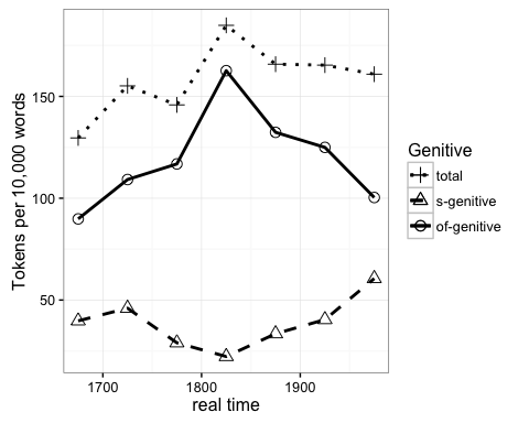
Figure 1. Mean interchangeable genitive frequencies (normalized to frequency per 10,000 words) by ARCHER period.
The advantage of this approach as opposed to the copying and pasting of results should be obvious. The latter approach requires that we manually update the statistics, tables, and figures every time we update our data or an element of the data analysis. This process is not only tedious and labor-intensive (imagine having to reproduce all the results six months to a year later based upon a reviewer’s suggestions) but also error-prone. It is not always easy to keep track of the results we have dropped into the document and whether those results are consistent with the most current form of the data and the data analysis. There is a very good chance that the reported results are simply inaccurate because they reflect an earlier stage of either the data or the data analysis. In the approach advocated here, there is no question of this document becoming out-of-sync with the data analysis pipeline that generated the results included within it, since the results are dynamically (re)produced whenever this document is generated. All the results that appear in the document necessarily reflect the most current form of the data and data analysis. The two aspects of published work – the generation of empirical results and the interpretation of those results – are thus both conceptually and physically united in that they both appear in the same form of representation.
Video 3. Demonstration of R Markdown.
A toy data analysis could incorporate all the R code and interpretative narrative in a single document. Most analyses, however, are considerably more complex than toy examples, insofar as they involve several distinct data analysis pipelines that perform conceptually distinct operations involving two or more datasets. Gathering data is a different process from cleaning it, cleaning data is a different process from creating new variables from existing ones, creating new variables is a different process from visualizing or modelling the data. While it is theoretically possible to write a single document that incorporates all the code that gathers and cleans the data, creates new variables, runs all the statistical models, and creates the resulting figures, tables, and graphs, such a document is difficult for authors to create and maintain and for readers to navigate and interpret.
One way around this problem is to limit the amount of operations a pipeline (and the source code that implements it) performs. A modular pipeline is one that is centered on a single operation or a few operations that are conceptually related to one another. One source code file would be responsible for performing one or just a few tasks. Header comments provide readers with essential information about the file. [13] Such information could include:
Here, for instance, is the example header for a file used in this project:
#----------------------------------------------------------------------------------------
# File: 03-recode-datives.R
# Author: Wolk et al. (rewritten by Joseph Flanagan)
# email: joseph.flanagan@helsinki.fi
# Purpose: Recode the datives dataset for Wolk et al.'s analysis
#----------------------------------------------------------------------------------------
# Uncomment following if you want to run just this script
# source("munge/01-download-data.R")
# source("munge/02-recreate-raw-data.R")
Once the code has been modularized, the next step is to make the links between the files explicit. It should go without saying that that files should all go into a single directory. In that way, sharing the project is simply a matter of sending a zipped file. The organization of the subdirectories and the naming of files can also aid in reproducibility. Files that should be run in a particular order should be numbered accordingly. Conceptually distinct files should be placed in different subdirectories. When calling files, one should avoid commands that require intervention by the user (for instance, using file.choose() to input a data file in R) and instead write the file name directly (e.g. read_csv("data/raw-data/archer-genitives.csv"). When writing the file names, it is preferable to use relative rather than absolute links (as in the preceding example). That way, the code is not dependent upon the particular file organization of a particular computer.
The image below shows how the files in this project have been organized:

Figure 2. Example project directory tree.
Data has been placed in the data/ directory, with raw-data/ containing that data in its original form, processed-data/ containing the data that has been modified from the original. Custom scripts are found in the lib/ directory. Scripts concerned with gathering and reshaping the data are found in the munge/ directory. They are numbered in the order they should be run. Scripts that perform the actual analysis – whether a model or a figure – are found in the R/ directory. The R Markdown file and accompanying .bibtex file are found in the documents/ directory, along with the final output generated from the R Markdown file, whether it be html, Word, or pdf. The R Markdown file is configured so that all figures that are included in the html, Word, or pdf documents are automatically stored in the figures/ directory. A README file (not shown in the diagram) provides necessary information about the project, including how to reproduce it.
Even with a logical directory structure, it might not be clear how the files relate to one another. As we have seen time and again, manually documenting the relationship among the files in a project places the same information in two different representational formats, with all the accompanying problems of keeping the two in sync. As we have also continually seen, it is better to have documentation and organization in the same representational format so that the dependencies among the files are instantiated in code: that way, reproducing the dependencies is simply a matter of re-running the code. This project is organized using the R package ProjectTemplate so that when the R Markdown file is rendered, custom scripts are first loaded, then the scripts in the munge/ directory are run in sequential order, then whatever files in the R directory are needed for the analysis. A GNU Make file makes it possible to generate output simultaneously in html, Word, and pdf formats. Someone interested in the project could thus reproduce all the component parts of the project, as well as the paper itself.
Video 4. Demonstration of the R package ProjectTemplate.
We have already seen the necessity of keeping track of all the changes that were made to the data during the course of analysis. This section is concerned with keeping track of changes made to the code. Strictly speaking, preserving the various stages of development code went through during the course of an analysis is not a requirement for reproducible research: in order to reproduce the analysis, one needs the code that ran the analysis, not an earlier stage of that code. Still, systematically archiving previous versions of the code aids in the reproducibility of the analysis in several ways. First, it provides a history of the project so that it is possible to know what changes were made, when, and by whom. Second, it allows someone to reproduce an earlier form of the analysis. This is especially helpful if it is necessary to revert to an earlier version of the code or data if a problem is discovered (e.g., the code gets broken, a file gets deleted, or raw data gets overwritten).
In order to keep track of changes in a systematic manner, it is necessary to store our data and code in a system that has version control. Microsoft Word has a simple form of version control in its Track Changes feature. (Obviously, this feature only works with Word documents). Dropbox keeps snapshots of all changes made to a file stored on its system for thirty days (Dropbox Pro subscribers have access to the Extended Version History feature, which stores snapshots for a year). These features are relatively easy to use, but they are limited in what they accomplish.
For this reason, it is probably better to use a version control system like Git. For those unfamiliar with Git, you can imagine it as combining the Track Changes features of Microsoft Word with a backup system like Dropbox or Apple’s Time Machine. You keep your work in a repository (or “repo” for short). Like Dropbox, the repository can be stored locally (on one or more machines) and on a remote server. As you make change changes to files within the repository, you periodically stage those changes and then commit them to the repository, adding a little note about what changes you made since the last commit (like Track Changes features in Microsoft Word). You can push changes from the local repository to the remote repository, or, alternatively, pull changes from the remote repository to the local in order to keep the repositories on different machines in sync. Each repository is thus a complete and self-contained copy of the project, with a log of all the changes made by the people who contributed to the project over the course of its development.
Git was developed for professional software designers, and it thus has an extensive feature set. The videos provide a brief introduction for how to use a small subset of those features for reproducible academic research. For an extensive introduction to Git, see Chacon & Straub (2014).
Now that we have taken steps to make our project reproducible, the final step is to make that project accessible by others. Among all the strategies discussed here, this strategy has been the one that has attracted the most support. Over the years, it has increasingly become common for researchers to provide pre-prints of articles, data, and even code for their projects. Still, the system has evolved in a very incoherent manner, such that the published article may appear in one location, the pre-print in another, the data in yet another, and the code in yet another. Spreading the various components of this project across multiple locations in this manner makes reproducibility both inconvenient and difficult. As we have continually seen in this paper, keeping the same information in two or more representations increases the likelihood of error. Perhaps a dataset gets updated in one location but the code does not. Perhaps the documentation of the code or the form of the data reflects an earlier stage of the project than those that led to the results published in the article. Perhaps the results in the article are inaccurate due to errors in the dataset or code that were only discovered after the article was published. Spreading the project across multiple locations raises an obvious question: Which form of the project is the “correct one?” We tend to privilege the published article (see below) but that is due more to tradition than a concern for accuracy.
In the interest of space, I shall only briefly mention what I consider the best option: storing the project on a cloud-hosting service based on the Git version control system. There are two such services already available: Bitbucket and Github. Both of these services were developed for software designers rather than for the dissemination of academic research, but, as seen throughout this paper, designing a reproducible research project is not so very different from designing a software package. Of the two, Github is by far the more popular, but Bitbucket may be more advantageous for academics because it offers free unlimited private and public repositories for academic users and teams. (Github offers academics only five private repositories.)
Given that reproducibility is supposedly one of the hallmarks of science, coupled with the fact that the tools for reproducible research are free and freely available, the fact that it is not possible to reproduce most of the results published in academic articles should be surprising. There are, however, a number of factors that make most researchers reluctant to share data and code. Borgman (2010: 196) cites four general factors: the lack of incentives (hiring and promotion is decided on the basis of the number of published articles, not for making research reproducible); the amount of effort and time required to make the work reproducible; the desire to keep data to oneself until one has squeezed all the research possibilities out of it; fear of losing control over intellectual property. In a survey of 723 American researchers, Stodden (2010a: Table 9, 20) found that the most common reasons for not sharing data and code were the generally the same as those cited by Borgman (2010). (Stodden also found that the second most common reason for not sharing code was the desire to avoid dealing with questions about the code.) Within the humanities, we could add that a lack of programming skills has led to a reliance upon GUI tools that make it difficult, if not impossible, to make results reproducible. Clearly, if we wish to make it easy and convenient to reproduce one another’s results, we have to address these factors, and change the system so that reproducibility is the norm rather than an option. [14] Finally, it is important to remember that simply because a work is reproducible doesn’t mean that it is correct. [15] Indeed, problems in the analysis arising from p-hacking, researcher degrees of freedom, or what Gelman & Loken (2014) refer to as “garden of forking paths” cannot be corrected by making data and code freely available, although it might make it possible to identify some of those problems. I thus consider the ability to reproduce results in the sense described in this paper only as the minimal standard for scientific work.
In closing, I would like to suggest that changing academic culture will involve a concurrent change in the way academic research is viewed. Perhaps the chief reason we tend to take the results published in articles largely on faith is due to the way in which academic culture has fetishized the published article to such an extent that it has become synonymous with research itself. Again, there may be some academic fields where article and research are more or less the same, but that is hardly the case for any kind of empirical research. In this regard, it might be helpful to think of the idea propagated by Buckheit & Donoho (1995):
An article about computational science in a scientific publication is not the scholarship itself, it is merely advertising of the scholarship. The actual scholarship is the complete software development environment and the complete set of instructions which generated the figures.
Of course, for much work outside of the computational sciences, we cannot make such a tight connection between the software and the actual scholarship as suggested in this quote, as there are more important considerations for the validity of a study than the fact that it is reproducible or not. As I mention above, the fact that a paper is reproducible does not mean that it is correct. Whether the findings of a particular study are robust is ultimately a question of data collection, study design, correct measurement of the variables, choice of statistical models, and other factors. Still, I would like us to consider the need to to elevate the current status of data and code as second class citizens within academic culture, so that we can more effectively evaluate the factors that do contribute to the validity of a particular study. More journal editors need to follow the example of Biostatistics and promote the reproducibility in the work they publish. [16] We need a means of recognizing the contribution of work that does not fit neatly into the current system of measuring academic worth on the basis of the “impact factor” of the journal it was published in or in the number of times the work was cited. [17] It is thus not until we take a much more expansive view of academic research that we will create an environment where the incentive to produce accurate results that can be reproduced by others will outweigh the incentive to publish as many articles as possible, no matter what errors they might contain. In short, the path to creating an academic culture in which reproducibility is not an added feature but an essential component of academic scholarship requires that we downgrade the status of articles and think of them as merely as what they are: advertisement for the repo.
[1] Carey provides the code used for calculating his figures at http://www.helsinki.fi/englanti/elfa/downloads/BASE_laughter_analysis_v2.py and http://www.helsinki.fi/englanti/elfa/downloads/ELFA_laughter_analysis_v2.py. [Go back up]
[2] This sense of “reproducibility” differs from how the term is used by, say, The Reproducibility Project: Psychology, where the term refers not to the ability to generate the same results by using the same data and code but to the ability to derive the same results as the original study using different data (but following the specifications of data collection as described in the original study). I follow Peng (2011) in referring to the latter as “replication”. For a discussion about how the terms reproducibility and replicability are currently used this context, see Liberman (2015). [Go back up]
[3] See Gandrud (2015) and Stodden, Leisch & Peng (2014) for more extensive discussions. Sandve et al. (2013) provide ten steps for reproducible research in the computational sciences, which parallels the discussion here. [Go back up]
[4] The code and data can be found at http://www.benszm.net/datasets/WBRS_data_June-30-2017.zip. [Go back up]
[5] This difficulty, by the way, probably explains why Nesi never provided an explanation for the mistaken word count. I suspect that she acted interactively with the data using GUI drop-down menus that do not automatically record the user’s actions, and thus she has no idea herself how the mistake occurred. [Go back up]
[6] This is related to the philosophy guiding Emacs Speaks Statistics (ESS): “the source code is real” (§12.4). [Go back up]
[7] See Martin (2008) for an extensive discussion. [Go back up]
[8] See, for instance, the discussion on “lme4 and languageR compatibility error” at Stack Overflow. [Go back up]
[9] Another approach would be to use the R package Checkpoint. [Go back up]
[10] See Xie (2015) for an in-depth discussion about how R Markdown is incorporated in the R package knitr. [Go back up]
[11] I have not worried about the styling of the document, as this will necessarily vary. However, it is possible to format the document in a manner consistent with most publishers’ requirements. [Go back up]
[12] The actual text reads “Consider the definiteness of the possessor. The default level of this factor is “`r as.character(genitives$definitenessPossessor[1])`”: given two contexts identical but for their definiteness classification, one being definite and the other a proper name, the model estimates a so-called “odds ratio” of e \textsuperscript `r round(coef(summary(genitive.model))["definitenessPossessordefinite-propername", "Estimate" ], digits = 2)` = `r round(exp(1) ^ coef(summary(genitive.model))["definitenessPossessordefinite-propername", "Estimate" ], digits = 2)`. That is, vis-à-vis a definite noun, a proper name is only `r round(exp(1) ^ coef(summary(genitive.model))["definitenessPossessordefinite-propername", "Estimate" ], digits = 2)` times as likely to appear in the of-genitive”. [Go back up]
[13] As we shall see in the next section, version control provides additional information, including when the file was last modified. [Go back up]
[14] Stodden (2010b) provides some recommendations about how to do so in the computational sciences. [Go back up]
[15] See Leek & Peng (2015). [Go back up]
[16] Peng (2009) describes the steps taken by the journal in this regard. [Go back up]
[17] An anonymous reviewer of this paper, for instance, suggested that I include a list of software packages mentioned in this paper. Insofar as academic credit is mainly conferred on the basis of citation counts, this is an important suggestion. However, more than sixty packages were used in this analysis, when package dependencies are taken into account. That is far too high a number to include in a list of references, especially in print journals where references are included in the total character count allowed in the paper. [Go back up]
This paper’s repository on Bitbucket: https://bitbucket.org/jflanaga/d2-e-proceedings/overview
The code and data used in this article, from Wolk et al. (2013): http://www.benszm.net/datasets/WBRS_data_June-30-2017.zip
Bitbucket: https://bitbucket.org
The British Academic Spoken English corpus (BASE): http://www2.warwick.ac.uk/fac/soc/al/research/collections/base
Discussion on “lme4 and languageR compatibility error” at Stack Overflow: http://stackoverflow.com/questions/19199713/lme4-and-languager-compatibility-error-input-model-is-not-a-mer-object
Emacs Speaks Statistics (ESS): http://ess.r-project.org/Manual/ess.html
Github: https://github.com
Google’s style guide for R: https://google.github.io/styleguide/Rguide.xml
Hadley Wickham’s style guide for R: https://cran.r-project.org/web/packages/formatR/formatR.pdf
The Michigan Corpus of Academic Spoken English (MICASE): http://quod.lib.umich.edu/cgi/c/corpus/corpus?c=micase;page=simple
Pandoc-flavoured Markdown: http://pandoc.org/README.html
R Markdown: http://rmarkdown.rstudio.com
R package Checkpoint: http://blog.revolutionanalytics.com/2015/01/reproducibility-with-revolution-r-open-and-the-checkpoint-package.html
R package formatR: https://cran.r-project.org/web/packages/formatR/formatR.pdf
R package Packrat: https://rstudio.github.io/packrat/. Ushey, Kevin, Jonathan McPherson, Joe Cheng, Aron Atkins & JJ Allaire. 2016. Packrat: A Dependency Management System for Projects and Their R Package Dependencies. https://CRAN.R-project.org/package=packrat
R package ProjectTemplate: http://projecttemplate.net. White, John Myles. 2016. ProjectTemplate: Automates the Creation of New Statistical Analysis Projects. https://CRAN.R-project.org/package=ProjectTemplate
The Reproducibility Project: Psychology: https://osf.io/ezcuj/wiki/home/
Allaire, JJ, Joe Cheng, Yihui Xie, Jonathan McPherson, Winston Chang, Jeff Allen, Hadley Wickham, Aron Atkins & Rob Hyndman. 2016. Rmarkdown: Dynamic Documents for R. http://rmarkdown.rstudio.com
Biber, Douglas, Edward Finegan & Dwight Atkinson. 1994. “ARCHER and its challenges: Compiling and exploring a representative corpus of historical English registers”. Creating and Using English Language Corpora: Papers from the Fourteenth International Conference on English Language Research on Computerized Corpora (Language and Computers), ed. by Udo Fries, Gunnel Tottie & Peter Schneider, 1–14. Atlanta: Rodopi.
Borgman, Christine L. 2010. Scholarship in the Digital Age. Information, Infrastructure, and the Internet. Cambridge, MA: MIT Press.
Buckheit, Jonathan B. & David L Donoho. 1995. “WaveLab and reproducible research”. Wavelets and Statistics (Lecture Notes in Statistics 103), ed. by A. Antoniadis & G. Oppenheim, 55–81. New York: Springer. doi:10.1007/978-1-4612-2544-7_5
Carey, Ray. 2013. “Laughter in academic talk: Brits, Yanks, and ELF compared”. https://elfaproject.wordpress.com/2013/07/27/laughter-in-academic-talk-brits-yanks-elf-compared/
Carey, Ray. 2014a. “A closer look at laughter in academic talk: A reader response”. Journal of English for Academic Purposes 14: 118–123. doi:10.1016/j.jeap.2014.03.001
Carey, Ray. 2014b. “Adventures in correcting the (semi-)scientific record”. https://elfaproject.wordpress.com/2014/11/25/adventures-in-correcting-the-semi-scientific-record/
Chacon, Scott & Ben Straub. 2014. Pro Git. 2nd edn. https://git-scm.com/book/en/v2
Gandrud, Christopher. 2015. Reproducible Research with R and RStudio. 2nd edn. Boca Raton, FL: Chapman & Hall/CRC.
Gelman, Andrew & Eric Loken. 2014. “The statistical crisis in science”. American Scientist 102(6): 460. doi:10.1511/2014.111.460
Knuth, Donald E. 1992. Literate Programming (CSLI Lecture Notes 27). Stanford, CA: Center for the Study of Language and Information.
Leek, Jeffrey T. & Roger D. Peng. 2015. “Opinion: Reproducible research can still be wrong: Adopting a prevention approach”. Proceedings of the National Academy of Sciences 112(6): 1645–1646. doi:10.1073/pnas.1421412111
Liberman, Mark. 2015. “Replicability vs. reproducibility – or is it the other way around?”. http://languagelog.ldc.upenn.edu/nll/?p=21956
Martin, Robert C. 2008. Clean Code: A Handbook of Agile Software Craftsmanship. 1st edn. Upper Saddle River, NJ: Prentice Hall PTR.
Nesi, Hilary. 2012. “Laughter in university lectures”. Journal of English for Academic Purposes 11(2): 79–89. doi:10.1016/j.jeap.2011.12.003
Nesi, Hilary. 2014. “A closer look at laughter in academic talk: A response to Carey (2014)”. Journal of English for Academic Purposes 15: 48–49. doi:10.1016/j.jeap.2014.07.001
Pedersen, Ted. 2008. “Empiricism is not a matter of faith”. Computational Linguistics 34(3): 465–470. doi:10.1162/coli.2008.34.3.465
Peng, Roger D. 2009. “Reproducible research and Biostatistics”. Biostatistics 10(3): 405–408. doi:10.1093/biostatistics/kxp014
Peng, Roger D. 2011. “Reproducible research in computational science”. Science 334(6060): 1226–1227. doi:10.1126/science.1213847
R Core Team. 2016. R: A Language and Environment for Statistical Computing. Vienna, Austria: R Foundation for Statistical Computing. https://www.R-project.org/
RStudio Team. 2015. RStudio: Integrated Development Environment for R. Boston, MA: RStudio, Inc. http://www.rstudio.com/
Sandve, Geir Kjetil, Anton Nekrutenko, James Taylor & Eivind Hovig. 2013. “Ten simple rules for reproducible computational research”. PLoS Computational Biology 9(10): e1003285. doi:10.1371/journal.pcbi.1003285
Stodden, Victoria. 2010a. “The scientific method in practice: Reproducibility in the computational sciences”. SSRN Electronic Journal: 1–33. doi:10.2139/ssrn.1550193
Stodden, Victoria. 2010b. “Reproducible research: Addressing the need for data and code sharing in computational science”. Computing in Science Engineering 12(5): 8–12. doi:10.1109/MCSE.2010.113
Stodden, Victoria, Friedrich Leisch & Roger D. Peng. 2014. Implementing Reproducible Research. Boca Raton, FL: Chapman & Hall/CRC.
Wolk, Christoph, Joan Bresnan, Anette Rosenbach & Benedikt Szmrecsanyi. 2013. “Dative and genitive variability in Late Modern English: Exploring cross-constructional variation and change”. Diachronica 30(3): 382–419. doi:10.1075/dia.30.3.04wol
Xie, Yihui. 2015. Dynamic Documents with R and Knitr. 2nd edn. Boca Raton, FL: Chapman & Hall/CRC. http://yihui.name/knitr/