Studies in Variation, Contacts and Change in English
Studies in Variation, Contacts and Change in English
Seth Mehl
University of Sheffield
Analysing strength of lexical co-occurrence using Mutual Information (MI) and Pearson’s chi-square test is standard in corpus linguistics; typically, such analyses are conducted using a statistical baseline of all tokens in the data set (cf. Manning & Schuetze 1999). That is, the probability of a given type or lemma is measured as the number of occurrences of that type or lemma against the total number of tokens in the data. This baseline, however, is not ideal as a measure of linguistic probability: the denominator representing all tokens is artificially high because each token does not represent an opportunity for the given lemma to occur (cf. Wallis 2012). This high denominator in turn results in an artificially low probability and suggests an artificially high degree of confidence in the measurement. This paper reports an experiment in employing a grammatical part of speech (POS) baseline for calculating statistical probability of co-occurrence, asking: In what ways does a POS-baseline differ from a traditional baseline of all tokens, when calculating chi-square and MI? The experiment is conducted in the context of a major research project studying meaning through lexical co-occurrence in Early Modern English texts, and the data is drawn from Early English Books Online (Text Creation Partnership edition). I demonstrate that the traditional baseline of all tokens yields higher MI values and more ‘significant’ results than a POS-baseline. I argue that the traditional baseline of all tokens can be interpreted as yielding artificially high MI values; and as yielding an artificially high number of significant results – but I also illustrate that the improvements of the POS-baseline may be negligible for the typical task of ranking the top ten co-occurrence pairs for a given node word.
The Linguistic DNA (LDNA) project, begun in 2015, has aimed to model meaning in Early English Books Online (Text Creation Partnership edition, EEBO-TCP) by analysing lexical co-occurrence, simultaneously and at scale, for all content lemmas in the collection’s approximately 1.2 billion tokens, across nearly 60,000 Early Modern English texts (cf. Fitzmaurice et al. 2017). The goal from the outset was to identify co-occurrence patterns for the mass of data, rather than for a small set of selected words; to calculate strength of lexical co-occurrence for all co-occurring content lemmas across the totality of the data; and to rank significant co-occurrences for the research team to investigate further through manual semantic and pragmatic analysis in co-text. To do this, the LDNA team, including members in the University of Sheffield’s Digital Humanities Institute (DHI), designed a bespoke computational linguistic tool for analysing the very large data set, and for producing the big data outputs representing co-occurrence patterns for every content lemma in the texts. Researchers determined early in the project that two approaches, standard in the field, would be employed to analyse lexical co-occurrence: Mutual Information (MI) and hypothesis testing with Pearson’s chi-square. MI scores are commonly used to rank co-occurring lexical pairs; and chi-square scores are commonly used to determine whether a co-occurring pair is likely to have occurred by chance. Both approaches rely on measures of probability, and here the team took the opportunity to reassess traditional approaches, asking: how do we measure the probability that two words co-occur in text?
In this paper, I first describe and explain MI, based in particular on Fano’s (1960) initial presentation of MI, and then describe and explain hypothesis testing with Pearson’s chi-square. I discuss some possible approaches to analysing probability in language, and some of the approaches to MI and chi-square which are not generally employed. Indeed, the range of alternative statistical baselines generally remains quietly unexamined (though for careful examinations, see Mehl 2018; Aarts et al. 2013; Wallis 2012). I then describe the LDNA project’s use of a grammatical baseline – specifically a Part of Speech (POS) baseline – for calculating statistical probability of co-occurrence. I argue that this grammatical POS-baseline reflects linguistic probability more meaningfully than traditional measures (cf. Fitzmaurice et al. 2017; Wallis 2012). I report the results of a pilot experiment comparing this grammatical baseline to the more established approach of counting all tokens as the baseline for probability of co-occurrence. I demonstrate that the LDNA POS-baseline produces considerably different results from the traditional baseline, and I argue that the traditional baseline of all tokens can be interpreted as yielding artificially high MI values; and as yielding an artificially high number of ‘significant’ results. I conclude that further testing of the POS-baseline is warranted, across a range of other calculations and variables, as it can be expected to improve results for quantitative linguistic research more broadly.
Mutual Information is a measure devised by Fano (1960: 21–31) in his seminal book on information theory, Transmission of Information. MI is defined by comparing a conditional probability to a non-conditional probability:
In corpus linguistics, we interpret the numerator as the probability of word b, given condition a. Specifically, this is generally the probability that word b occurs within a given proximity of word a. The LDNA project interprets the denominator of the equation as the general unconditioned probability of word b occurring in the corpus – the LDNA project’s interpretation of this denominator is atypical for corpus linguistic applications, but is built on the first principles of Fano’s (1960: 27) description of MI. [1] A full discussion of the various instantiations of the denominator is beyond the scope of the present paper, but we argue that our approach is theoretically sound, and firmly based in Fano’s (1960) original formulations.
MI thus compares the probability that word b occurs near word a; to the probability that word b occurs anywhere in the data. Specifically, MI takes the log base 2 of this equation:
This log allows the MI score to be interpreted in terms of ‘bits’ of information (Manning & Schuetze 1999: 179). An MI score of zero reflects that the probability of word b occurring near word a is the same as the probability of word b occurring anywhere in the text, i.e. ‘the two events in question are statistically independent’ (Fano 1960: 28). Put differently, this means that the presence of word a provides no additional information on the likelihood of word b occurring nearby. A positive MI score indicates that word b is more likely to occur near word a than in the text in general; and a negative MI score indicates that word b is less likely to occur if word a is present (Fano 1960: 28). [2] MI scores can be interpreted as a measure of strength of co-occurrence: the highest MI scores indicate that word b is much more likely to occur near word a than in the corpus in general. The scores are thus typically used to rank lexical co-occurrences from the pairs that are most strongly connected, to the pairs that occur roughly as often near each other as anywhere else.
MI is sometimes said to be sensitive to, or weighted towards, low-probability events. This can be understood by considering a given word b that occurs only once. If its only occurrence is near word a, then the probability of its occurrence within the proximity of a is extremely high; if the data is large, like that of EEBO-TCP, then the probability of word b occurring in the data is extremely low. This contrast results in a very high MI score. Higher-frequency events are less likely to exhibit such a stark contrast. Because low-frequency events will tend to have higher MI scores, one of two options can be employed alongside MI: first, low-frequency words can be removed from the data entirely; second, MI can be used alongside hypothesis testing. Hypothesis testing is an appropriate technique alongside MI because it accounts not only for effect size (i.e. the contrast between word b occurring near word a,and word b occurring anywhere in the data), but also data size (including the raw frequency of occurrence of word b). Hypothesis testing can thus be used to remove those events that are so low frequency that we cannot be confident about generalizing our observations; remaining co-occurrences can then be ranked using MI. Hypothesis testing is explained further in the next section.
Hypothesis testing in corpus linguistics begins by formulating a null hypothesis that the population underlying a given sample of text is not essentially different from expectation (Sheskin 2003: 53–59). [3] When analysing lexical co-occurrence, the given sample is generally the text within a defined proximity of word a, measured in terms of the probability of word b occurring within that proximity; the value for ‘expectation’ is generally the probability of word b occurring in the corpus as a whole. It is thus parallel to the LDNA project’s application of MI described above. Put differently, the chi-square test hypothesises that the difference between the two probabilities is only what would be expected by chance between any two samples of the same population. The test calculates the probability that the two samples might be drawn by chance from the same population; and then rejects the null hypothesis if that probability is lower than a defined threshold (Manning & Schuetze 1999: 162–163).
Pearson’s chi-square test is commonly used for such hypothesis testing in linguistics (cf. Manning & Schuetze 1999: 162–163). [4] In measuring lexical co-occurrence, we generally start by counting the number of times that word b occurs within a given proximity of word a. We then consider the number of times that word b did not occur near word a: this should be understood as the number of times that word b could have occurred within the proximity of word a but did not actually occur. Moving on to expected values, we generally count the number of times that word b occurs in the corpus as a whole, and the number of times that word b could have occurred within the corpus as a whole, but did not occur. Obviously, these numbers relate to observations of a probability of occurrence similar to that described above in the discussion of MI (to be discussed further below). These values are generally presented as a contingency table, as follows:
| Proximity around a | Entire corpus | |
|---|---|---|
| Instances of word b | O1 | E1 |
| Instances in which word b could have occurred but did not | O2 | E2 |
Table 1. A contingency table presenting values used in Pearson’s chi-square test when analysing lexical co-occurrence.
The equation for calculating chi-square scores is as follows:
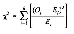
The equation’s results are checked against a table of chi-square scores to determine significance at a given threshold.
As noted above, rejection of the null hypothesis is related to both the effect size and the size of the data. The effect size can be understood as the size of the difference between the two observed probabilities (the probability of b occurring within a proximity of word a, and the probability of b occurring anywhere in the data), which, again, is conceptually parallel to MI. The size of the data is related to the observed probability of occurrence, and it can be understood as the number of times that word b is seen to occur as well as the number of times that it is seen to have been able to occur (but did not). The more data we have, and the larger the effect size, the more confident we can be in our observation. With a very large amount of data, the test will suggest that even a very small effect size represents an essential difference from expectation. In fact, this can be a pitfall of big data, and also causes problems for hypothesis testing in corpus linguistics when using a baseline of all tokens, as I discuss below.
It is clear that both MI and Pearson’s chi-square relate to measures of probability, and that a probability, properly understood, is a measure of how many times an observation occurs, against a measure of how many times it could have occurred (cf. Wallis 2012). For probabilities around flipping coins or rolling dice, this is straightforward: we count the number of times that a coin lands heads up, out of the total number of times that we flipped the coin. How do corpus linguists generally approach probability? Typically, probabilities of lexical co-occurrence are measured using a statistical baseline of all tokens in the data set (cf. Manning & Schuetze 1999: 170; Church & Hanks 1990: 23). That is, the probability of a given word b is measured as the number of occurrences of word b out of the total number of tokens in the data N.
However, the denominator or baseline N is not ideal as a measure of linguistic probability for the simple reason that N will rarely, if ever, be equal to the number of times that word b could occur. This fact can be understood from two perspectives. First, it is not the case that each word in a text could have been word b; i.e. each word in the text could notbe replaced with word b. Second, it is not the case that all words in a text could have been word b; i.e. all words in the text cannotbe replaced with word b. This denominator N,representing all tokens, is thus artificially high because each and every token does not represent an opportunity for the given lemma to occur (cf. Wallis 2012). If N is artificially large, it renders the probability b/N artificially low. Applied to the chi-square test, this high denominator also suggests that we have more data about word b than we actually have – i.e. that we have actually counted N instances where word b could have occurred but did not – which, in a chi-square test for hypothesis testing, falsely indicates high confidence in the probability itself. That is, we artificially suggest that the data size is very large, and thus, even small differences in effect size can be interpreted as essential or significant.
What alternative baselines might we consider? In the most general and fundamental sense, we can consider any quantifiable element of language: syllables, morphemes, words, phrases, clauses, semantic or pragmatic units, and so on. For lexical occurrence, it is sensible to employ a baseline that is some measure of words. There are at least two well-documented alternatives to the baseline of all tokens, for measuring probabilities of lexical occurrence. One option is to analyse probabilities in relation to semantic alternations. This approach is definitive of onomasiological semantic research. Geeraerts et al. (1994) describe the onomasiological approach tidily, in relation to linguistic probability, asking: given that a language user is expressing a concept x, what is the probability that the language user employs word b or c (or d, e, and so on)? An onomasiological baseline thus reflects the psycholinguistic process whereby a language user (consciously or unconsciously) selects an option (in this case a word) for expressing a given meaning (Geeraerts et al. 1994; Wallis 2012). In this case, we understand each instance of word b or c to be a possible instance of word b; that is, each instance of word c could be replaced by word b, and in fact all instances of word c could be replaced by word b. This onomasiological approach yields a realistic probability measure, reducing or eliminating invariant Type C terms (Wallis 2012), i.e. those non-alternates that result in an inflated denominator. On the other hand, it has also been argued that these types of alternation studies – even when they include a wide range of alternates – generally fail to acknowledge the wide range of true alternates for expressing a given meaning, including not only lexical alternations, but grammatical variants, information packaging options, and broad pragmatic options; and also fall short in discerning the shades of complex contexts where alternation may in fact not be possible due, for instance, to pragmatic or social factors (cf. Smith & Leech 2013). It may be that most onomasiological alternation studies err on the side of reducing invariant terms, rather than exhaustively identifying true alternates.
An onomasiological alternation approach proved impossible for the LDNA project. The onomasiological approach requires a careful identification of semantic alternates. A primary aim of the LDNA project has been to map probabilities for lexical co-occurrences of all lemmas, at scale, across all of EEBO-TCP, so a careful identification of semantic alternates simply is not feasible. [6]
Another possibility is to analyse probabilities using syntactic information. Dependency models are becoming more common in Natural Language Processing, for automatic identification of synonyms or other related words (cf. Pado & Lapata 2007; Kilgarriff et al. 2014). These models identify a particular word in a specific syntactic relationship with another word, such as, for example, water as the Direct Object (DO) of drink. In this example, instead of identifying all instances of water and counting them in relation to the total number of tokens (or to the total number of synonyms for water as in onomasiological study), we count all instances of water as the DO of drink in relation to the total number of DOs of drink. This is a reasonable, if imperfect, probability measure. It would be unreasonable to suggest that each and every DO of drink (tea, coffee, beer, wine, etc.) could be replaced by water, but it is nonetheless indisputable that this approach reduces invariant Type C terms that certainly cannot alternate with water, but which would be included in a baseline of all words (including prepositions, verbs, and so on).
Dependency models, however, are not appropriate for the LDNAproject because automatic syntactic parsing of Early Modern English is simply too under-developed and therefore error-prone (cf. Hundt et al. 2012). To calculate probabilities at scale, automatic parsing is certainly necessary – and therefore dependency models such as this one are not possible for LDNA.
Neither an onomasiological baseline nor a syntactic baseline is feasible at scale with early modern data. In exploring other possible means for reducing invariant terms and calculating more realistic probability figures, it is necessary to consider the automatic annotation that is reasonably and reliably available for EEBO-TCP. Specifically, EEBO-TCP has been pre-processed for the LDNA project with a lemmatiser and POS-tagger (details below). It was decided that a reasonable alternative to onomasiological or syntactic baselines is a grammatical baseline. Precedent for use of a grammatical baseline can be found in grammatical research including Aarts et al. (2013), who measure instances of progressive verb phrases out of the total number of verb phrases. In fact, Aarts et al. (2013) compare their grammatical baseline to a ‘per million words’ baseline and analyse the differences in the results; that method can be seen as directly parallel to the experiment conducted here. Similarly, Bowie et al. (2013) measured instances of perfect verb phrases out of the total number of tensed, past-marked verb phrases, and compared their grammatical baseline to a ‘per million words’ baseline. Both of those studies, produced at the Survey of English Usage, can be seen as laying the groundwork for the grammatical baseline employed by the LDNA project.
The LDNA project’s grammatical baseline is a POS-baseline. The method identifies every instance of word b within proximity of word a, and counts it against every instance of the POS of word b within proximity of word a. We then identify every instance of word b in all of EEBO-TCP, and count it against every instance of the POS of word b in all of EEBO-TCP. We use this approach for calculating both MI and chi-square.
The LDNA POS-baseline is not perfect: it is certainly problematic to suggest that each noun can alternate with any other noun, or with all other nouns. But, we argue that this approach is nonetheless much stronger than suggesting that each noun can alternate with any other token, or with all other tokens. Moreover, it is certain that employing a POS-baseline dramatically reduces invariant Type C terms. We therefore theorise that it should produce more realistic probability measures, by reducing the artificially inflated denominators of the N baseline, and thus minimise the problem of artificially low probabilities and the suggestion of artificially large data size. As a result, the POS-baseline should reduce the problem of artificially high MI and chi-square scores.
A pilot experiment was conducted to compare the LDNA processor’s POS-baseline to the traditional N baseline, and to gauge the differences between the outputs. It was decided that co-occurrences would be analysed for all content lemmas. To render this pilot experiment manageable, co-occurrence data is therefore limited to two texts selected from EEBO-TCP: Speed’s History of Great Britaine (1611; TCP ID A12738); and Boyle’s Considerations touching experimental natural philosophy (1663; TCP ID A29031). The two texts represent the later period of EEBO-TCP, which presents less spelling variation than earlier texts, resulting in fewer problems for lemmatisation and POS-tagging (see below). The two texts also represent two different genres (history and science, respectively); and two different text lengths: Speed’s History at 725,000 tokens and Boyle’s Considerations at c180,000 tokens. This was deemed a reasonable scope for the pilot study. While observed co-occurrences are only calculated within each text, respectively, expected values are derived from the probability of occurrence of each lemma in EEBO-TCP as a whole, with the POS-baseline and the N baseline.
The two texts were first pre-processed using MorphAdorner (Burns 2013), for lemmatisation and POS-tagging. MorphAdorner is designed specifically for Early Modern English, and MorphAdorner v2.0 is the tool that underlies Chadwyck’s search interface for EEBO-TCP. Our data has been processed using a new and as yet publicly unavailable MorphAdorner v3.0, which was then subject to manual corrections by the MorphAdorner team (personal communication 2018, Martin Mueller). This data therefore represents the state of the art in Early Modern English text cleaning and preparation for corpus linguistic analysis. It was decided that co-occurrences would be analysed for all noun, verb, and adjective lemmas; that is, each noun, verb, or adjective lemma is counted as a node, and all co-occurrences between each node and each co-occurring noun, verb, or adjective lemma is then counted and indexed. The restriction to nouns, verbs, and adjectives allows a focus on content lemmas, rather than grammatical ones such as prepositions and conjunctions. It might have been ideal to include adverbs as well, but, as a peculiarity of MorphAdorner’s tagging system, adverbs are grouped into a macro-category entitled ‘adverbs, particles, and conjunctions’ (Burns 2013). This category includes a very large number of grammatical words, which is not ideal for this experiment. It is also so large as to cause problems for the principle of the POS-baseline: the POS-baseline is intended to reduce Type C invariant terms. The macro-category of ‘adverbs, particles, and conjunctions’ does not satisfy that logical requirement.
Co-occurrence pairs were analysed across proximity windows of +/-5, 10, 30, and 50 tokens, to the left and right of each node. A window of +/-5 tokens is typical in corpus linguistic research. Because the LDNA project is particularly interested in discursive co-occurrences, our default processing has been +/-50 tokens, with the aim of studying a coherent discursive span somewhat akin to a paragraph in present day written English (cf. Fitzmaurice et al. 2017). Windows of +/-10 and +/-30 have been calculated for this experiment in order to provide a more comprehensive analysis between the standard +/-5 token window and the unusual LDNA +/-50 token window.
MI and chi-square were calculated using the LDNA processor, for all co-occurring pairs of noun, verb, or adjective lemmas; across all proximity windows; using the POS-baseline and the N baseline.
The POS-baseline yields overall lower MI values than the N baseline. That is, using the POS-baseline, more MI scores generally suggest that the probability of word b occurring within the given window around word a is closer to the probability of word b occurring in the corpus as a whole. This is in line with the hypothesis that the POS-baseline should effectively lower otherwise artificially high MI scores. The mean difference between MI scores calculated with the N baseline and the POS-baseline at each proximity window are presented in Table 2.
| Proximity window | Speed’s History | Boyle’s Philosophy |
|---|---|---|
| +/-5 tokens | 5.75 | 5.54 |
| +/-10 tokens | 7.77 | 7.55 |
| +/-30 tokens | 10.95 | 10.72 |
| +/-50 tokens | 12.42 | 11.46 |
Table 2. Mean difference in MI scores between N baseline and POS-baseline.
MI scores are between approximately 5 and 13 points higher using the N baseline than the POS-baseline. Example histograms are presented below, showing the distribution of MI score differences between the N baseline and the POS-baseline for each text, at the smallest and largest proximity windows. The middle proximity windows distribute similarly.
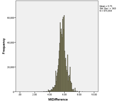
Figure 1. Histogram of differences in MI scores between N baseline and POS-baseline (calculated as N baseline minus POS-baseline) for all pairs in Speed’s History with a proximity window of +/-5 tokens.
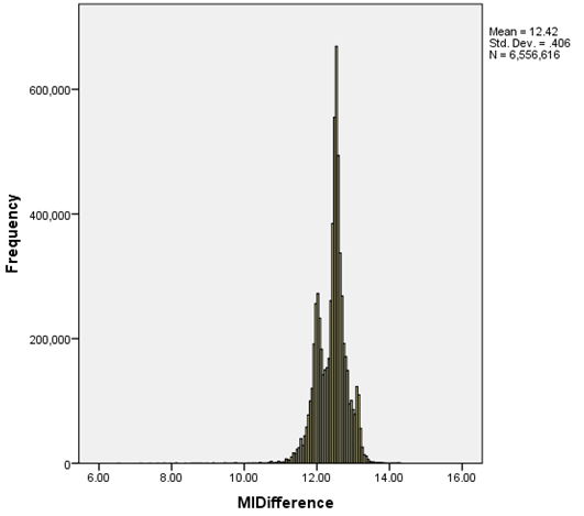
Figure 2. Histogram of differences in MI scores between N baseline and POS-baseline (calculated as N baseline minus POS-baseline) for all pairs in Speed’s History with a proximity window of +/-50 tokens.
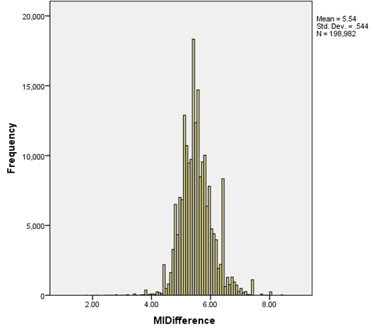
Figure 3. Histogram of differences in MI scores between N baseline and POS-baseline (calculated as N baseline minus POS-baseline) for all pairs in Boyle’s Considerations with a proximity window of +/-5 tokens.
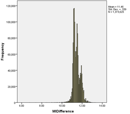
Figure 4. Histogram of differences in MI scores between N baseline and POS-baseline (calculated as N baseline minus POS-baseline) for all pairs in Boyle’s Considerations with a proximity window of +/-50 tokens.
The highest MI differences are observable in the larger text, Speed’s History, at the largest proximity window, +/-50 tokens. As an illustration, some examples of lemma pairs with the highest MI differences in this text are displayed in Table 3, below.
| Lemma A | Lemma B | MI (N baseline) | MI (POS-baseline) | MI difference |
|---|---|---|---|---|
| ordovices | monmouth | 23.3 | 9.1 | 14.2 |
| montgomery | nottingham | 23.3 | 9.1 | 14.2 |
| penbrookshire | westmoreland | 23.9 | 9.7 | 14.2 |
| caermarden | worcestershire | 25.4 | 11.2 | 14.2 |
| merch. | island | 19.1 | 4.9 | 14.2 |
Table 3. Example lemma pairs that exhibit high differences between MI (N baseline) and MI (POS-baseline) in Speed’s History.
Some pair co-occurrences have positive MI scores with a baseline of all words but negative MI scores with the POS-baseline. In most systems, negative MI scores would be removed from the data; the POS-baseline thus potentially produces considerably different outputs from the N baseline. Pairs that have positive MI scores with the N baseline but negative MI scores with the POS-baseline are presented in Table 4, as a percentage of all pairs in each data set, and as raw numbers. As can be seen in the table, the POS-baseline could result in the loss of thousands or even hundreds of thousands of pairs, compared to the N baseline, depending on the size of the data being analysed. Again, we can see this as reducing artificially high MI scores.
| Window | Speed’s History | Boyle’s Philosophy |
|---|---|---|
| +/-5 | 5% (52,291 pairs) | 4% (7,620 pairs) |
| +/-10 | 7% (124,153 pairs) | 5% (17,797 pairs) |
| +/-30 | 9% (426,514 pairs) | 6% (60,444 pairs) |
| +/-50 | 9% (901,587 pairs) | 7% (102,254 pairs) |
Table 4. Pairs that have positive MI scores with N baseline but negative MI scores with POS-baseline, as a percentage of all pairs, and as a raw number.
As is apparent in Table 4, the largest differences in this regard appear in Speed’s History, with a proximity window of +/-50 tokens.Some examples of lemma pairs that have positive MI scores with the N baseline but negative MI scores with the POS-baseline in Speed’s History are shown in Table 5.
| Lemma A | Lemma B | MI (N baseline) | MI (POS-baseline) |
|---|---|---|---|
| king | moses | 5.1 | -7.6 |
| duke | apostle | 6.0 | -6.7 |
| be | ministry | 5.8 | -6.7 |
| French | christ | 6.1 | -6.6 |
| daughter | soul | 6.4 | -6.4 |
Table 5. Example pairs that have positive MI scores with N baseline but negative MI scores with POS-baseline, in Speed’s History, at a proximity window of +/-50.
MI scores are generally used to rank co-occurrences; the N baseline and POS-baseline exhibit considerably different rank orders. Table 6 displays the mean rank order difference between the POS-baseline and the N baseline. The mean change in rank order (calculated across all pairs) is a shift of between approximately 62,000 and 1.2 million for the longer text (depending on the window size), and between approximately 9,000 and 278,000 for the shorter text.
| Window | Speed’s History | Boyle’s Philosophy |
|---|---|---|
| +/-5 | 62,427 | 9,105 |
| +/-10 | 198,888 | 37,062 |
| +/-30 | 448,768 | 163,103 |
| +/-50 | 1,225,679 | 278,639 |
Table 6. Mean rank order difference for all pairs.
Specific rank order differences for each text at the largest and smallest window sizes are presented in the histograms below, as examples. The middle window sizes distribute similarly. There is a very large number of pairs whose rank order change is very small, but as is apparent in the histograms, there is a tail with a second mode that is in fact very high, in all instances.
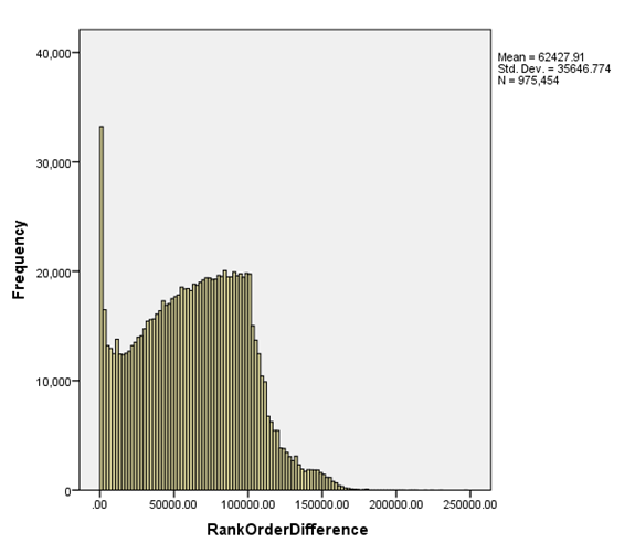
Figure 5. Histogram of MI score rank differences (calculated as absolute value of N baseline rank minus POS-baseline) for all pairs in Speed’s History with a proximity window of +/-5 tokens.
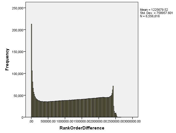
Figure 6. Histogram of MI score rank differences (calculated as absolute value of N baseline rank minus POS-baseline) for all pairs in Speed’s History with a proximity window of +/-50 tokens.
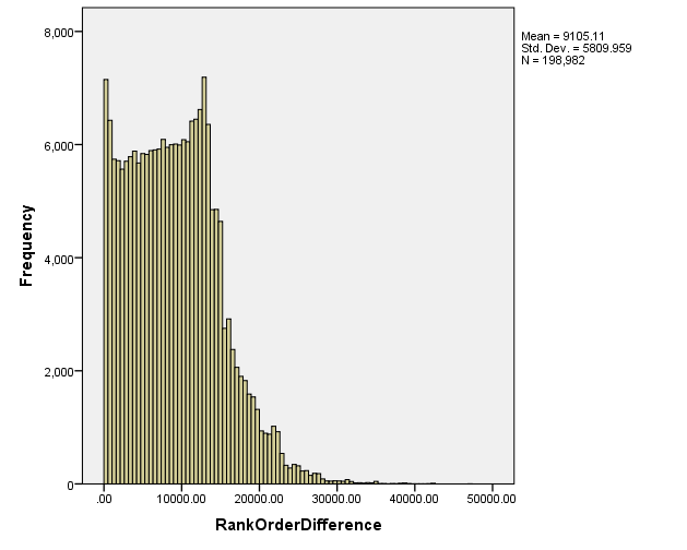
Figure 7. Histogram of MI score rank differences (calculated as absolute value of N baseline rank minus POS-baseline) for all pairs in Boyle’s Considerations with a proximity window of +/-5 tokens.
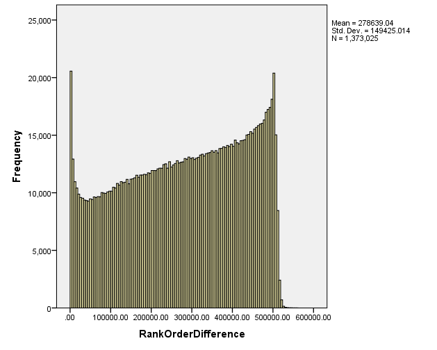
Figure 8. Histogram of MI score rank differences (calculated as absolute value of N baseline rank minus POS-baseline) for all pairs in Boyle’s Considerations with a proximity window of +/-50 tokens.
As an illustration, some examples of lemma pairs with large rank order differences are shown in Table 7, drawn from Speed’s History with a proximity window of +/-30.
| Lemma A | Lemma B | Rank (N baseline) | Rank (POS-baseline) | Rank order difference |
|---|---|---|---|---|
| musician | good | 1,038,432 | 2,671,359 | 1,632,927 |
| affable | great | 986,251 | 2,618,721 | 1,632,470 |
| speck | man | 816,135 | 2,429,117 | 1,612,982 |
| matt | god | 1,099,138 | 2,665,130 | 1,565,992 |
| richmondshire | time | 793,602 | 2,405,607 | 1,612,005 |
Table 7. Example pairs that have a large rank order difference between N baseline and POS-baseline, in Speed’s History, at a proximity window of +/-30.
Of course, MI scores are not often used to rank co-occurrences across all the millions of pairs of a text or a text collection; often, it is only the very strongest pairs that are of interest. Table 8 displays the mean rank order difference between the POS-baseline and the N baseline for the top 100 pairs in each text. Here, the mean change in rank order is a shift of between approximately 1 and 13 places in ranking.
| Window | Speed’s History | Boyle’s Philosophy |
|---|---|---|
| +/-5 | 0.89 | 3.24 |
| +/-10 | 1.89 | 5.11 |
| +/-30 | 2.01 | 10.35 |
| +/-50 | 1.57 | 12.91 |
Table 8. Mean rank order differences for top 100 pairs.
These relatively small rank order differences in the top 100 pairs are telling: it may be that for the most common use of ranking the top 100 or fewer pairs, the advantages of the POS-baseline are negligible. Moreover, MI is frequently used to rank co-occurrence pairs for individual node words, one at a time. Below, I present rank order differences for the top 12 pairs for a relatively low-frequency adjective (abject) and a medium-frequency noun (liquor), for the commonly used proximity window of +/-5 tokens, in Boyle’s Considerations.
| Lemma A | Lemma B | Pair rank (POS-baseline) | Pair rank (N baseline) |
|---|---|---|---|
| abject | reptile | 1 | 1 |
| abject | despicable | 2 | 2 |
| abject | loadstone | 3 | 3 |
| abject | bulk | 4 | 4 |
| abject | eagle | 5 | 6 |
| abject | obvious | 6 | 5 |
| abject | create | 7 | 12 |
| abject | property | 8 | 9 |
| abject | lion | 9 | 10 |
| abject | filthy | 10 | 7 |
| abject | instance | 11 | 11 |
| abject | vile | 12 | 8 |
Table 9. Rank order for the top 12 co-occurrences pairs with the node word abject, with POS-baseline and N baseline, in Boyle’s Considerations, proximity window +/-5 tokens.
| Lemma A | Lemma B | Pair rank (POS-baseline) | Pair rank (N baseline) |
|---|---|---|---|
| liquor | coc_-tree | 1 | 1 |
| liquor | lyantery | 2 | 2 |
| liquor | beccabunga | 3 | 3 |
| liquor | glasse-stopples | 4 | 4 |
| liquor | stolone | 5 | 6 |
| liquor | empyrema | 6 | 7 |
| liquor | barbada | 7 | 8 |
| liquor | glass-stopples | 8 | 5 |
| liquor | limphatick | 9 | 9 |
| liquor | reimbibe | 10 | 12 |
| liquor | distillable | 11 | 11 |
| liquor | alimbick | 12 | 10 |
Table 10. Rank order for the top 12 co-occurrences pairs with the node word liquor, with POS-baseline and N baseline, in Boyle’s Considerations, proximity window +/-5 tokens.
As is evident in Tables 9 and 10, the rank order difference for the top pairs of the given node words might be seen as negligible. This data, along with the data in Table 8, suggest that for such analyses of top co-occurrence pairs for a single node, the improvements offered by the POS-baseline may be negligible. It should also be noted that all of these pairs pass a chi-square test for significance with both the N baseline and the POS-baseline. That is not, however, the case for all the data.
Indeed, the N baseline yields higher chi-square scores, and more significant results at p<0.05, than the POS-baseline. With a baseline of all words, all pairs are significant at p<0.05. With a POS-baseline, only 72-86% of pairs are ‘significant’ at p<0.05, as displayed in Table 11.
| Window | Speed’s History | Boyle’s Philosophy |
|---|---|---|
| +/-5 | 82% (174,838 pairs) | 86% (170,446 pairs) |
| +/-10 | 78% (1,449,556 pairs) | 83% (316,086 pairs) |
| +/-30 | 74% (3,320,630 pairs) | 79% (741,168 pairs) |
| +/-50 | 72% (4,717,300 pairs) | 77% (1,058,608 pairs) |
Table 11. Percentage of all pairs that are deemed ‘significant’ at p<0.05, POS-baseline.
The observations in Table 11 are in line with the hypothesis that the artificially inflated denominator of the Nbaseline will suggest an artificially high data size, resulting in artificially high confidence in the observation and an artificially high number of ‘significant’ results. Table 12, below, lists example pairs that are significant with the Nbaseline, but not significant with the POS-baseline, in Boyle’s Considerations, with a proximity window of +/-5 tokens.
| Lemma A | Lemma B |
|---|---|
| person | show |
| great | promise |
| cure | give |
| oil | world |
| particular | find |
| body | white |
| use | reason |
| perform | think |
| part | infinite |
| pyrophilus | lay |
| look | come |
| furnace | take |
Table 12. Lemma pairs that pass a chi-square test for significance with the N baseline but not the POS-baseline.
I have demonstrated that a baseline of all tokens yields higher MI values than a POS-baseline, and that the baseline of all tokens yields more significant chi-square scores at p<0.05. I have in turn argued that the baseline of all tokens can be seen as yielding an artificially high number of significant results, and artificially high MI values. I would advocate broader experimentation with the POS-baseline as a theoretically sound approach to measuring lexical co-occurrence strength in big data.
How do we know if the results described here for the POS-baseline are in fact an improvement on an N baseline? I have argued that the POS-baseline is reasonable, based on a theoretical understanding of probability, and my theoretical framework has adequately predicted – at least within the scope of this pilot experiment – the differences that have been observed. The POS-baseline thus seems to be theoretically more sound than the N baseline. The results here confirm that the difference between the two baselines is considerable. It is therefore at least advisable to explore this difference, and its implications further.
I have also shown that for the typical practice of using MI to rank co-occurrence pairs for a single node, the improvements offered by the POS-baseline may be negligible. This finding is not applicable or the LDNA project, which has aimed to identify lexical co-occurrence patterns across millions of words, rather than for a small set of selected words or a specific node word. In addition, the LDNA project has aimed to assess these patterns at scale, rather than being limited only to strongest co-occurrences.
The present pilot experiment represents only a sliver of what is possible with the POS-baseline. Future experiments should examine larger data sets and a wider range of text types, including spoken language. Using other POS taggers, it will be reasonable to experiment with adverbs as an additional POS as well. While the present study has examined quantitative differences between the POS-baseline and the N baseline for MI and Pearson’s chi-square, future experiments might test the POS-baseline for other commonly used statistics in corpus linguistics, including log likelihood, log dice, PMI, and others. Future work could also test the POS-baseline within a range of larger computational linguistic approaches, including vector-based distributional semantic methods, which often employ MI at scale (or a variant such as normalised MI).
Future work could also evaluate the POS-baseline in other ways, including, for example, its ability to improve computational performance on synonymy tests, or its ability to match native speaker intuition about collocational, semantic, or discursive relationships. Such tests would allow us to assess whether the N baseline might be seen to yield ‘false positives’, which the POS-baseline eliminates. In order to do this, a definition of true or false positives would need to be determined, in relation, perhaps, to synonym tables or native speaker intuition, or in relation to other NLP tasks.
[1] MI has often been used in corpus linguistics to generate statistics for adjacent collocations (cf. Church & Hanks 1990; Bouma 2009), and the equation generally employed is an algebraic equivalent to Fano’s (1960: 28) first equation, written:
When applied to language data, with wide proximity windows, interpreting equation i becomes problematic. In particular, the numerator of equation i indicates the intersection of event a and event b. In corpus linguistics shorthand, this is often defined as the intersection of ‘word a’and ‘word b’, but corpus linguists are generally not, in fact, interested in a word that is both word a and word b. Instead, we are interested in the intersection of ‘word b’ and ‘the proximity around word a’. By this definition, the denominator must then be defined as the probability of ‘word b’ multiplied by the probability of ‘the proximity around word a’. Instead, corpus linguists most often define the denominator as the probability of ‘word b’ multiplied by the probability of ‘word a’. This discrepancy is non-trivial when analysing non-adjacent co-occurrences, as in the present study. The LDNA project is continuing to explore Fano’s (1960) original presentation of MI, alongside the range of more recent applications of MI and Pointwise Mutual Information (PMI; cf. Church & Hanks 1990), including multiple instantiations of and variations on the MI and PMI equations, and their theoretical foundations. Forthcoming publications will address this issue further. [Go back up]
[2] In corpus linguistics, negative MI scores are often discarded. The LDNA project has been exploring negative MI scores, and all positive and negative scores are counted in the experiment conducted for the present paper. [Go back up]
[3] I describe a single-sample chi-square test here, though any number of samples can be compared, as in what is known as a two-sample chi-square test or an RxC (row by column) chi-square test (cf. Sheskin 2003: 219, 493). [Go back up]
[4] This section is based largely on Sheskin (2003: 56–53, 219–223). [Go back up]
[5] In addition to the citations here, I am indebted to Sean Wallis for a great deal of extraordinarily valuable personal communication around these issues. [Go back up]
[6] More recently, the Semantic EEBO (or SEEBO) corpus has been created by the Historical Thesaurus of English team at Glasgow University (personal communication, 2018, Marc Alexander). The SEEBO corpus uses the SAMUELS semantic tagger to identify the semantic category of every word in EEBO-TCP. It may be possible in the future to measure probabilities of lexical occurrence using those semantic tags as a probabilistic baseline. [Go back up]
Aarts, Bas, Joanne Close & Sean Wallis. 2013. “Choices over time: Methodological issues in investigating current change”. The English Verb Phrase, ed. by Bas Aarts, Joanne Close, Geoffrey Leech & Sean Wallis. Cambridge: Cambridge University Press.
Bouma, Gerlof. 2009. “Normalized (pointwise) mutual information in collocation extraction”. From Form to Meaning: Processing Texts Automatically, Proceedings of the Biennial GSCL Conference, ed. by Christian Chiarcos, Richard Eckart de Castilho & Manfred Stede, 31–40. Tübingen: Gunter Narr.
Bowie, Jill, Sean Wallis & Bas Aarts. 2013. “The perfect in spoken British English”. The English Verb Phrase, ed. by Bas Aarts, Joanne Close, Geoffrey Leech & Sean Wallis. Cambridge: Cambridge University Press.
Burns, Philip R. 2013. “MorphAdorner v2: A Java library for the morphological adornment of English language texts”. Evanston, IL: Northwestern University.
Church, Kenneth Ward & Patrick Hanks. 1990. “Word association norms, mutual information, and lexicography”. Computational Linguistics 16(1): 22–29.
Fano, Robert M. 1960. Transmission of Information: A Statistical Theory of Communications. Boston: MIT Press.
Fitzmaurice, Susan, Justyna A. Robinson, Marc Alexander, Iona C. Hine, Seth Mehl & Fraser Dallachy. 2017. “Linguistic DNA: Investigating conceptual change in Early Modern English discourse”. Studia Neophilologica 89: 21–38.
Geeraerts, Dirk, Stefan Grondelaers & Peter Bakema. 1994. The Structure of Lexical Variation. Berlin: Mouton de Gruyter.
Hundt, Marianne, David Denison & Gerold Schneider. 2012. “Retrieving relatives from historical data”. Literary and Linguistic Computing 27(1): 3–16.
Kilgarriff, Adam, Vít Baisa, Jan Bušta, Miloš Jakubíček, Vojtěch Kovář, Jan Michelfeit, Pavel Rychlý & Vít Suchomel. 2014. “The Sketch Engine: Ten years on”. Lexicography 1: 7–36.
Manning, Christopher & Hinrich Schuetze. 1999. Foundations of Statistical Natural Language Processing. Boston: MIT Press.
Mehl, Seth. 2018. “What we talk about when we talk about corpus frequency: The example of polysemous verbs with light and concrete senses”. Corpus Linguistics and Linguistic Theory. doi:10.1515/cllt-2017-0039
Pado, Sebastian & Mirella Lapata. 2007. “Dependency-based construction of semantic space models”. Computational Linguistics 33(2): 161–199.
Sheskin, David J. 2003. Handbook of Parametric and Non-parametric Statistical Procedures. 3rd ed. Boca Raton, FL: CRC Press.
Smith, Nick & Geoffrey Leech. 2013. “Verb structures in twentieth century British English”. The Verb Phrase in English: Investigating Recent Language Change with Corpora, ed. by Bas Aarts, Joanne Close, Geoffrey Leech & Sean Wallis, 68–98. Cambridge: Cambridge University Press.
Wallis, Sean. 2012. “That vexed problem of choice”. London: University College London. http://www.ucl.ac.uk/english-usage/staff/sean/resources/vexedchoice.pdf