2 METHODS
2.1 Questionnaire
The survey questionnaire contained 49 questions, seven of which were used to gather background information on the respondents. The remaining questions focused on the respondents’ English language skills and use of English, plus their attitudes to English. The English translation of the questionnaire can be found as an appendix.
The background information collected in the questionnaire included the respondent’s gender, year of birth, area where the respondent had spent most of his/her childhood and adolescence, level of education, and occupation; also the size and monthly net income of the respondent’s household. The questions relating to English were grouped into six categories:
1. Languages in your life
This section covered the respondents’ own accounts of their general linguistic background: mother tongue, possible bi- or multilingualism, and the role of different languages in terms of studies and uses; also language contacts in the respondents’ environment.
2. English in your life
This section focused on English in particular, and on its significance in the lives of the respondents. The questions aimed at finding out e.g. where the respondents encountered English, how they viewed different varieties of spoken English, and how they viewed the position of English in Finland and elsewhere.
3. Studying and knowing English
The questions here related to respondents previous English studies and to self-evaluations of their English language skills. The respondents were asked e.g. how long they had studied English, how they viewed their skills in different areas of English, whether they felt their English skills were adequate, and where they had acquired their English skills.
4. Uses of English
This section aimed at extensive coverage of the respondents’ use of English, no matter how limited: it asked about the use of English in leisure time and at work (speaking, listening, writing, reading, and use of the internet), and about the reasons for using English. Respondents were also asked to evaluate various behaviours and emotions related to the use of English.
5. English alongside the mother tongue
This section focused on how respondents reacted to communication in which there was a mix of English and the mother tongue. In addition, the questions aimed at finding out how often, in what kind of situations, and for what reasons the respondents themselves mixed their mother tongue with English in their speech and writing.
6. The future of English in Finland
The last section of the questionnaire asked respondents to focus on the year 2027. Respondents were asked to predict the future status of English in Finland, which age groups, professions, etc. would have to be able to speak English, and in what respects Finns would miss out on something if they lacked skills in English. In addition, the respondents were asked to predict which language might compete with English for the status of the most important international language.
2.2 Sampling and data collection
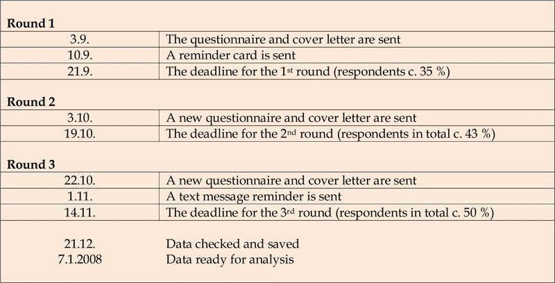
The research data were collected by drawing a random sample from the Finnish population database of Statistics Finland. The target population was defined as all Finnish citizens aged 15–79, with the exception of those living in the small Swedish-speaking island province of Åland. The size of the target population was 3.9 million people. The sampling design adopted was a stratified systematic sampling, where the strata consisted of four age groups 15–24, 25–44, 45–64, and 65–79. The sample size was allocated equally between the strata, i.e. the same number of people was sampled from each age group. To ensure the regional representativeness of the sample, the sampling frame (i.e. the target population) was sorted prior to sampling by the domicile code (which identifies the location of the domicile). The sample size was originally set at 3 000 people (750 persons per stratum). The data collection was conducted by Statistics Finland, via a postal questionnaire. The questionnaire, plus a covering letter, was posted in September 2007. Data collection took place from 1st September 2007 until 4th November 2007. The stages in the collection are shown in Table 3.
The final sample data set consisted of 1 495 respondents (approximately 50 % of the planned sample size). In the preliminary data analyses it was noted that the response activity varied strongly according to the gender, age, and residential area of the respondent. The response rate appeared highest (63 %) among women aged 55 years or over, and lowest (29 %) among men aged under 25. To correct the resulting distortion in the statistical analyses we used a weighting method based on post-stratification (Pahkinen & Lehtonen 1989; Lohr 1999). We divided the sample data into additional strata with respect to gender, residential province, and type (urban / semi urban / rural) of residential municipality. The final strata were then used to determine a corrective weighting for each individual in the sample. The new weighting calibrated the sample distributions of age, gender, province, and municipality type in such a way as to agree with the distributions in the
target population. The weightings were computed by Statistics Finland by CALMAR software (Deville & Särndal 1992) and scaled to add up to the observed sample size (Deville et al. 1993), i.e. 1 495. This meant that the average weighting was one, with the respondents who were overrepresented in the sample receiving a corrective weight of less than one, and conversely, those underrepresented in the sample receiving a corrective weight of more than one.
TABLE 3 The stages in the data collection and the number of respondents in each stage (2007–2008)
In statistical terms, the weighting based on post-stratification is appropriate if it can be assumed that the nonresponse is random in each stratum (Little & Rubin 2002). In other words, the reluctance to respond is assumed to depend only on the variables employed in the stratification (here: age, gender, province, and type of municipality) or else on matters not related to the survey questions, for example a lack of time or a general reluctance to take part in opinion polls. The response probability can be then assumed to be the same for all respondents in the same stratum (e.g. young men living in cities), regardless of how they might have answered the given questions (e.g. on how long they had studied English). If the assumption holds, within each stratum there will be no systematic distributional difference between the responders and non-responders, and the weighted sample will represent the target population well. The assumption is not always realistic, but if it holds even approximately, the survey results can be considered to be approximately unbiased.
The factors which in this survey could have had systematic effect on nonresponse would include, for example, the respondent’s level of education, skills in English, and attitude to the use of English. However, these can be considered at least moderately associated with the variables employed in the post-stratification, and especially with age and area of residence. We can thus infer that the weightings adopted will assist in correcting for biasing factors of this kind. In addition, we noted that the response rate increased almost linearly with age. Since we know that older Finnish people tend to know and use English less than the younger age groups, we can assume that the nonresponse rates observed in the study had no straightforward relation to weak English skills, or to a less active use of English.
In addition to the non-responders, many respondents returned the questionnaire with some questions unanswered. Overall, this item
nonresponse was low: item-specific response rates were in most cases at least 90 %. One can therefore assume that item nonresponse did not cause any major bias in the survey results. The lowest response rate was for Question 15, and particularly sub-item (b), which dealt with the negative feelings caused by different varieties of English. This item seemed to pose problems for some older and less educated persons, for whom English was not part of the everyday environment. Among the 65–79 age group, and among those whose education had advanced no further than primary school, the response rate for this sub-item fell below 70 % – the only instance of this kind in the questionnaire. In addition, in a few other questions (23, 27, 33, 34, and 37) certain sub-items had a nonresponse rate of below 80 %, again among older and less educated respondents. Apparently they found these questions, or their sub-items, irrelevant or difficult to answer, because of weak skills or minor use of English.
In many questions the nonresponse could arguably be equated with the options no opinion or never (in questions concerning the use of English). However, we did not recode the data or apply any missing data imputation methods, partly because constructing valid statistical models for data imputation was considered too laborious compared to the limited gains achievable. We believe that our survey data set, as included here, gives a fairly accurate picture of the English skills, use of English, and attitudes to English among the Finnish adult population.
2.3 Background variables
Most of the survey questions were transformed into statistical variables so that the options of the questions and the values of the statistical variables are in complete correspondence. However, in some questions with multiple polytomous items, the items were dichotomised (e.g. into agree–disagree, or into about once a week–less frequently). This was done to simplify the presentation of results and conclusions. The details of each dichotomisation are rigorously described in the following sections as the results are discussed.
TABLE 4 The gender distribution

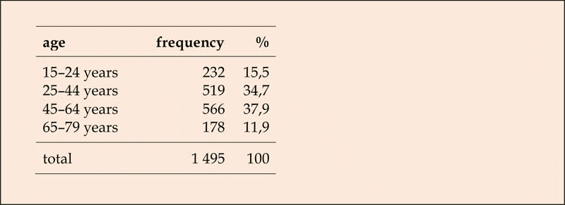
The distributions of the statistical variables were examined with respect to six background variables: gender, age, area of residence, education, occupation and monthly net income. In the case of missing values the questionnaire data on gender and age were replaced with the relevant official data available for all respondents from the database of Statistics Finland. The age groups used in the analyses were those used as strata: 15–24, 25–44, 45–64, and 65–79 years. The distributions of gender and age are shown in Tables 4 and 5.
TABLE 5 The age distribution
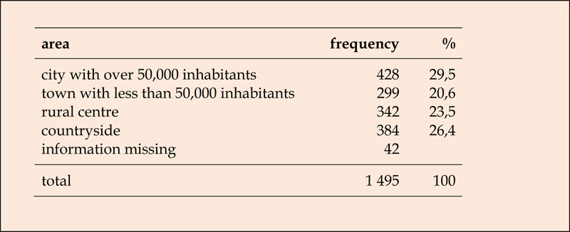
The questionnaire asked about the type of neighbourhood in which the respondent had spent most of his/her childhood and adolescence. However, in the data analyses we preferred to consider the respondent’s current place of residence rather than the childhood neighbourhood. For this purpose a new variable was extracted from the database of Statistics Finland. This consisted of four residential classes: (1) city with over 50,000 inhabitants, (2) town with less than 50,000 inhabitants, (3) rural centre, (4) countryside. The distribution of this variable is presented in Table 6. If we compare the residential distribution with the distribution for childhood neighbourhood (Table 7) (even though the classifications are not exactly equivalent) we clearly see that the population is moving to cities. For instance, out of those respondents who had spent their childhood and adolescence in the countryside, 47 % now live in a city or town. Conversely, out of those respondents who had spent their childhood and adolescence in a city or town, only 19 % now live in a rural centre or countryside.
TABLE 6 The residential distribution
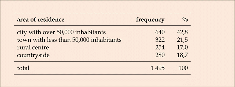
TABLE 7 The residential distribution of during childhood and adolescence
Question 46 asked about the respondent’s education using a five-point scale: (1) primary school (grades 1–6 in the Finnish system), (2) lower secondary school (grades 7–9/10 in the Finnish system), (3) upper secondary school or vocational education, (4) polytechnic degree, and (5) university degree. The five-point scale was used in the distribution analysis without recategorisation. The response rate was 97 %, and the distribution is shown in Table 8.
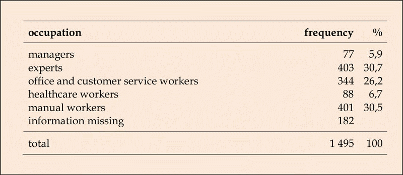
Question 47 asked about the respondent’s occupation. Here, 16 different occupational groups were presented (see questionnaire). Respondents were asked to choose the group to which they belonged at the time when they were last working. The response rate was 85 %. Out of those who did not respond, 70 % were young people who had not yet entered working life. For the purposes of the data analysis five main occupation categories were formed: (1) managers, (2) experts, (3) office and customer service workers, (4) healthcare workers, and (5) manual workers. The distribution thus obtained is shown in Table 9.
TABLE 8 The educational distribution
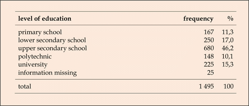
TABLE 9 The occupation distribution
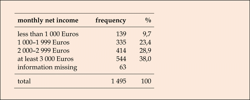
Question 49 asked about the monthly net income of the respondent’s household. A four-point scale was used: (1) less than 1 000 Euros, (2) 1 000–1 999 Euros, (3) 2 000–2 999 Euros, and (4) at least 3 000 Euros. In this question the response rate was 95 %, and the four-point scale was used without recategorisation. The distribution is shown in Table 10.
The background variables chosen are strongly correlated with each other. This means that analyses with respect to the various background variables may yield overlapping information. Education, occupation, and income are obviously associated with each other: managerial and expert duties typically require a high level of education, and the salaries of such occupations are typically high. In this survey, 80 % of the managers belonged to the highest income group, and 57 % had at least a polytechnic degree. The respective proportions among experts were 54 % and 63 %. Only 5 % of manual workers were included in the highest income group and 25 % had at least a polytechnic degree. In view of this, we decided to omit the income considerations from the final report, since their results could essentially be reduced to the results obtained from education and occupation.
TABLE 10 The distribution of the monthly net income per household
The data set also reveals a clear correlation between gender and occupation: 69 % of managers and 78 % of manual workers were men, whereas 73 % of office and customer service workers and 90 % of healthcare workers were women. Place of residence was particularly related to education and occupation. The cities showed particularly clear differences from other neighbourhoods: 24 % of the respondents living in a city had a university or a polytechnic degree, whereas in other areas this proportion was less than 10 %. In addition, 40 % of the respondents living in a city worked as experts, whereas in the other areas the proportion of experts varied from 19 % to 28 %. Only 19 % of the respondents from the cities were manual workers, whereas in the other residential areas the proportion of manual workers was at least a third, reaching as high as 47 % in the countryside. Moreover, in the countryside the proportion of respondents with a low level of education was remarkably high: 41 % of the respondents had been educated no further than lower secondary school. In the other areas the corresponding proportion fell between 23 % and 30 %.
2.4 Statistical analyses
As mentioned in Section 2.2, in the statistical analyses weights based on post-stratification were employed to get results that would be as representative as possible, in the light of the available information. Because the main aim of our data analyses was to produce merely descriptive information on the distributions of the survey variables, and to study them with respect to the most important background variables, we did not carry out any imputation of missing data. Hence, the percentages of the survey variables were computed from the observed data with no modification other than the weights, as previously described. The weighting of observations means that in determining frequency distributions, the observed frequency of each value is replaced with the sums of the weights for the observations in question.
In this study, the percentage distributions were examined both in the total data and in the subgroups determined by gender, age, residential area, education and occupation. Because the sample was stratified by age group and post-stratified by gender and residential area (in our case by province and municipality), we can expect that in these subgroups our statistical conclusions will be reliable (provided that the nonresponse is approximately random). With respect to education and occupation, the representativeness of the data may be weaker; however, since these variables bear a relation to age, gender, and area of residence, we can infer that the stratification and weighting will also improve the reliability of the conclusions regarding education and occupation.
The associations of the survey variables were tested by the chi-square test for two-way tables, and in some cases by Fisher’s exact test (e.g. Wonnacott & Wonnacott 1990). The association was considered to be statistically significant if the observed p value was under or close to the familiar 5 percent level. The overall data set is large enough to permit high statistical power for the tests (except for some analyses of certain small subgroups). Thus we anticipate that the methods adopted can identify with high probability the associations existing in the target population. Nevertheless, due to the large size of the data set, it is possible that the tests may find differences which are statistically significant, but which are of no practical importance in terms of our aims for this study. In the following sections where results are discussed, these issues are considered within every analysis before conclusions are drawn.
The results of the chi-square test are always approximate. The validity of the chi-square analysis requires that the variables should have a sufficient number of observations in every category considered. The established rule for the validity of the chi-square test is that none of the expected cell frequencies in the two-way tables may be less than one, and with at most 20 % of the cell frequencies being less than five (Wonnacott & Wonnacott 1990). When this condition does not hold, an indication is given in the corresponding result table.
All the statistical analyses were carried out by SPSS software, version 15, and by SAS software, version 9.1 for the Windows environment.
Back to top
|

